REVIEW 4 major objections 4 minor 45 references
Active galactic nucleus time-variability analysis and its caveats
T0 review · 4 major / 4 minor · reviewed 2026-08-11 · deepseek-v4-flash
Pith's one-line read Flare-biased sampling distorts the power spectra of AGN light curves, and standard simulations that reuse the observed time stamps cannot reproduce the distortion.
desk verdict Useful caveats review with two simulation-based findings, but the flare-bias claim needs error bars and a null ensemble before it carries weight. read the letter →
The pith
A machine-rendered reading of the paper's core claim, the machinery that carries it, and where it could break.
The reading
What carries the argument
The load-bearing object is the periodogram computed after linear interpolation of an unevenly sampled light curve, together with the PSRESP simulation procedure that copies the observed time stamps onto simulated light curves, and the EMP13/IAAFT surrogate-data iteration that is supposed to match a specified probability density function. Interpolation smooths over gaps, reducing high-frequency power and steepening the periodogram; the paper's simulations show that when dense sampling is aligned with flares, this steepening is partly cancelled because the flares themselves are well resolved, whereas randomly placed dense-sampling windows in simulations are not. The EMP13 algorithm's iterative step also acts as a phase-randomising operation, and the paper shows that cutting the simulated series before that step mixes the red-noise leak into the periodogram in a way that windowing cannot undo.
What would settle it
Measure the correlation between observing-cadence density and flux density in a monitoring data set, then compare the observed periodogram with the PSRESP-simulated mean periodogram: if a source with strong flare-biased sampling shows no systematic offset, or if a source with zero sampling-flux correlation still shows the mismatch, the flare-bias explanation would be wrong. A simpler simulation check is to generate a light curve with a known PSD, apply a deliberately flare-biased sampling pattern, and verify the predicted sign and size of the offset; removing the flare-sampling correlation should make the offset disappear.
Extended reading notes
Core claim
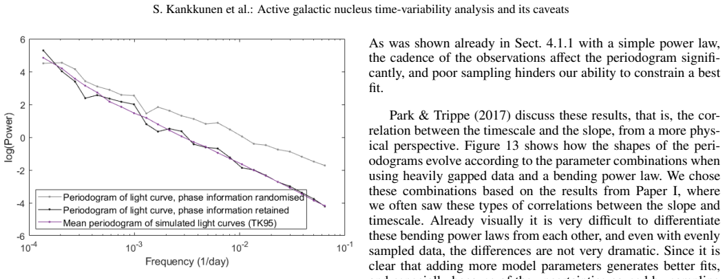
The central discovery is a mismatch between observed and simulated periodograms that traces to the correlation between sampling density and source brightness. In the PSRESP method, the observed sampling pattern is copied onto simulated light curves so that sampling artefacts appear in both, and the goodness of fit is judged by comparing the observed periodogram with the simulated mean periodogram. The authors simulate a flare-biased observing pattern and find that the real flare-biased light curve, after interpolation, yields a periodogram that is steeper than the evenly sampled case but not as steep as the mean periodogram of simulations carrying the same time stamps. The reason is that in the simulations the dense-sampling windows fall randomly with respect to flares, whereas in the actual flare-biased light curve they preferentially fall on the flares, suppressing the smoothing effect of interpolation. The same mechanism, the paper argues, can make a single observed light curve look significantly different from its own simulations even when the underlying PSD model is correct. The paper's second discovery is that the EMP13 surrogate algorithm loses phase information when its long initial simulation is cut to the observing-window length before the iterative step, which prevents Hann-window or end-matching corrections from removing red-noise leak and flattens the periodogram for steep PSD slopes.
Load-bearing premise
The claim depends on real monitoring campaigns being genuinely denser during flaring states, coupled with the absence of that coupling in simulations that merely reuse the time stamps; the paper illustrates the effect with simulated flare-biased sampling and notes that its own radio data shows much less prominent flare bias, but does not measure the correlation's strength in actual AGN data.
Editorial extensions
If this is right
- For sources whose monitoring cadence is correlated with flaring, PSRESP model fits will systematically compare the observed periodogram to a simulation ensemble that is biased in the opposite direction, so inferred PSD slopes and bend timescales carry an error not captured by the fit's scatter.
- A large parameter space of good fits is to be expected in sparsely sampled periodogram fitting; slope and characteristic timescale are strongly correlated and cannot be pinned down from such data.
- The EMP13 shortcut of cutting the light curve before the iterative step flattens periodograms of steep-spectrum sources, making it impossible to put reliable upper limits on PSD slopes when windowing is used.
- The Hann window and end-matching correct red-noise leak only when phase information is preserved; quasiperiodicity searches that use windowing on phase-randomised surrogates can produce false detections or false non-detections.
- The Lomb-Scargle false-alarm probability applies only to white noise and should not be used to claim quasiperiodicities in red-noise AGN data.
Reading between the lines
- The flare-bias mechanism should apply to any stochastic astronomical source observed with a target-of-opportunity or alert-driven cadence, not just AGNs; X-ray and gamma-ray transients and microlensing events could show the same observed-versus-simulated periodogram mismatch.
- A direct empirical test would be to measure the cross-correlation between observing density and flux state in a real monitoring data set and check whether the observed-minus-simulated periodogram offset scales with that correlation.
- Papers that report bend timescales from PSRESP on sparsely sampled radio light curves may need re-analysis with flare-bias-aware simulations; the authors note their own radio data has much less prominent flare bias, so the effect may be most relevant to X-ray and optical campaigns with flare-triggered follow-up.
- The EMP13 phase-randomization issue suggests that published surrogate-based significance estimates for quasiperiodicities, especially for steep PSD slopes, could shift if the full-length iterative step is used; re-running such analyses would be a cheap check.
Editorial analysis
A structured set of objections, weighed in public.
Referee Report
Summary. The paper presents a practical review of statistical caveats in AGN variability analysis, supported by simulations. It reproduces known issues (red-noise leak, aliasing, interpolation effects, structure function biases) and claims two previously overlooked caveats: (1) interpolation of light curves whose sampling is biased toward flaring states affects the measured PSD differently than applying the same sampling times to independent simulated light curves, thereby biasing PSRESP-style fits; and (2) the EMP13 surrogate algorithm is often misused when the light curve is cut to a shorter segment before the iterative step, because this randomizes phase information and prevents windowing from correcting red-noise leak. The paper also discusses periodogram normalisation, timescale estimation, and quasiperiodicity detection, and it summarises lessons learned from the authors' companion Paper I.
Significance. If the flare-bias claim holds, it would affect a broad class of PSD fitting studies of AGN light curves, particularly in radio monitoring where sampling density may correlate with flaring activity. The EMP13 caveat is a useful practical warning for surrogate-data users. The paper is valuable as a consolidated review with simulation-based demonstrations, and the authors are appropriately cautious about some limitations of their own tests. However, the statistical evidence for the main new claim is currently insufficient, so the central novelty is not yet established.
major comments (4)
- [§4.1.1, Fig. 3] The central claim that flare-biased sampling changes the effect of interpolation on the PSD is supported only by a visual comparison between a single periodogram (black) and the mean of 1000 simulated periodograms (purple), with no error bars, quantile ranges, or significance test. Because red-noise periodograms have large realization-to-realization scatter, the apparent difference could be a fluctuation. Please provide the distribution of the simulated periodograms (e.g., 5–95% percentiles) or, ideally, the distribution of single-realization periodograms under the null hypothesis that the sampling times are independent of the flux values, and state explicitly whether the observed black periodogram lies outside that null distribution.
- [§4.1.1] The construction of the flare-biased sampling is described only qualitatively ('dividing the time stamps of flux densities into two arrays based on their values'), which makes it impossible to reproduce or assess the magnitude of the bias. Please specify the exact algorithm, including the selection rule, the density contrast between flaring and non-flaring states, the interpolation scheme used, and the parameter values for the simulation shown in Fig. 3. Without this, the generality of the claimed effect cannot be evaluated.
- [§4.1.1 and §7] The paper notes that the MRO light curves have 'much less prominent' flare bias but never defines or measures flare bias in real data. To make the practical claim actionable, the authors should propose a quantitative metric for the correlation between sampling density and flux level, report it for the simulations, and, if possible, for the MRO data. Otherwise the relevance of the effect to actual AGN monitoring campaigns remains speculative.
- [§5.4.2, Figs. 11–12] The claim that cutting the TK95 light curve before the EMP13 iterative step randomizes phase and hence disables windowing-based red-noise-leak correction is demonstrated only by example light curves and periodograms. Please add a quantitative comparison across multiple realisations (e.g., mean and scatter of measured PSD slopes with and without phase preservation) and state the range of β for which the effect is significant. As written, the reader cannot tell whether the effect is large enough to affect typical AGN analyses.
minor comments (4)
- [§5.1, Eq. (8)] Please define ΔPsim(ν) explicitly; from the text it is presumably the standard deviation of the simulated periodograms, but the notation is ambiguous.
- [§4.1.2, Fig. 5] The comparison of normalisation schemes is based on one example; it would be helpful to state over how many simulations the 'closer' agreement was assessed.
- [§5.4.1] The statement that TK95 variance does not depend on N is imprecise; the variance of the simulated series does depend on the number of points through the normalization of the Fourier components. Please clarify the intended meaning, particularly in relation to the red-noise-leak simulation lengths.
- [§6.1, Fig. 13] The correlation between β and the bend timescale is shown visually but not quantified; a simple measure of overlap of the periodogram distributions or a summary statistic would strengthen the claim.
Circularity Check
No significant circularity; the paper is a transparent simulation study whose caveat claims do not reduce to fitted inputs or self-citations.
full rationale
The paper's central claims are produced by controlled simulations with known input PSD/PDF models, not by fitting parameters and then predicting the same data. The flare-bias finding (Sect. 4.1.1, Fig. 3) is constructed by generating timestamps correlated with flux density in one light curve and applying the same timestamps to independent realizations; the paper explicitly explains that the difference arises because 'the replicated periods of denser sampling only randomly occur during flares in simulated light curves.' This is a transparent, by-design demonstration of a mechanism rather than a hidden circularity: no quantity is fitted from one part of the data and then reported as a prediction of another part. The EMP13 phase-randomization caveat (Sect. 5.4.2, Figs. 11-12) is likewise demonstrated by comparing simulation choices; the conclusion follows from the algorithm description but is independently exhibited numerically. Self-citations to Paper I provide model parameters, slopes, and context (Sects. 1, 2.2, 4.1.1, 6), but none of these citations are load-bearing for the abstract's new caveats; the new results stand on the simulations reported in this paper. The absence of error bars on the mean simulated periodogram in Fig. 3 is a statistical robustness concern, not a circularity concern. Overall, the derivation chain is empirical and self-contained; no equation reduces to its own input, and no fitted parameter is renamed as a prediction.
Assumptions & free parameters
free parameters (3)
- Flare-bias strength and selection rule =
not quantified
- Simulated PSD parameters (beta and xb) =
e.g., beta = 2, xb = 500 days
- Red-noise-leak simulation length multiplier =
10 (up to 10,000 tested)
assumptions (4)
- domain assumption AGN light curves can be modeled as realizations of stochastic processes with simple or bending power-law PSDs.
- standard math The periodogram is an approximately unbiased estimator of the underlying PSD when binned or averaged.
- domain assumption The TK95 and EMP13 algorithms produce valid realizations of the target PSD and PDF when used according to their original prescriptions.
- ad hoc to paper Observations of AGNs can be biased toward flaring states, meaning sampling density correlates with flux density.
Cite this review
Pith. "Pith review of Active galactic nucleus time-variability analysis and its caveats." pith.science (2026). https://pith.science/paper/UBVH7QJX
@misc{pith2026241208192,
  author       = {Pith},
  title        = {Pith review of: Active galactic nucleus time-variability analysis and its caveats},
  year         = {2026},
  howpublished = {\url{https://pith.science/paper/UBVH7QJX}},
  note         = {Machine review of arXiv:2412.08192}
}
read the original abstract
In this study, we demonstrate some of the caveats in common statistical methods used for analysing astronomical variability timescales. We consider these issues specifically in the context of active galactic nuclei (AGNs) and use a more practical approach compared to mathematics literature, where the number of formulae may sometimes be overwhelming. We conducted a thorough literature review both on the statistical properties of light-curve data, specifically in the context of sampling effects, as well as on the methods used to analyse them. We simulated a wide range of data to test some of the known issues in AGN variability analysis as well as to investigate previously unknown or undocumented caveats. We discovered problems with some commonly used methods and confirmed how challenging it is to identify timescales from observed data. We find that interpolation of a light curve with biased sampling, specifically with bias towards flaring events, affects its measured power spectral density in a different manner than those of simulated light curves. We also find that an algorithm aiming to match the probability density function of a light curve has often been used incorrectly. These new issues appear to have been mostly overlooked and not necessarily addressed before, especially in astronomy literature.
Figures


Figures from the paper (10 more)



Reference graph
Works this paper leans on
-
[1]
Belloni, T. & Hasinger, G. 1990, A&A (ISSN 0004-6361), vol. 227, no. 2, Jan. 1990, p. L33-L36., 227, L33
work page 1990
-
[2]
Deeming, T. J. 1975, Ap&SS, 36, 137
1975
-
[3]
& Nandra, K
Edelson, R. & Nandra, K. 1999, ApJ, 514, 682
1999
-
[4]
Emmanoulopoulos, D., McHardy, I., & Papadakis, I. 2013, MNRAS, 433, 907
work page 2013
-
[5]
Emmanoulopoulos, D., McHardy, I. M., & Uttley, P. 2010, MNRAS, 404, 931
work page 2010
-
[6]
Fougere, P. F. 1985, J. Geophys. Res.: Space Physics, 90, 4355
work page 1985
- [7]
-
[8]
Heinzel, G., Rüdiger, A., & Schilling, R. 2002, Max Plank Inst, 12
work page 2002
Show all 45 references
-
[9]
2007, A&A, 469, 899
Hovatta, T., Tornikoski, M., Lainela, M., et al. 2007, A&A, 469, 899
2007
-
[10]
1992, ApJ, Part 1 (ISSN 0004-637X), vol
Hughes, P., Aller, H., & Aller, M. 1992, ApJ, Part 1 (ISSN 0004-637X), vol. 396, no. 2, Sept. 10, 1992, p. 469-486., 396, 469
1992
-
[11]
Hunt, G. A. 1956, Trans. Am. Math. Soc, 81, 294
1956
-
[12]
C., Bechtold, J., & Siemiginowska, A
Kelly, B. C., Bechtold, J., & Siemiginowska, A. 2009, ApJ, 698, 895
2009
-
[13]
C., Becker, A
Kelly, B. C., Becker, A. C., Sobolewska, M., Siemiginowska, A., & Uttley, P. 2014, ApJ, 788, 33
2014
-
[14]
Keshner, M. S. 1982, Proc. IEEE, 70, 212 Kozłowski, S. 2016, MNRAS, 459, 2787 Lähteenmäki, A., Järvelä, E., Hovatta, T., et al. 2017, A&A, 603, A100
1982
-
[15]
A., & Abbt, M
Limpert, E., Stahel, W. A., & Abbt, M. 2001, Biosci., 51, 341
2001
-
[16]
J., Türler, M., Valtaoja, E., et al
Lindfors, E. J., Türler, M., Valtaoja, E., et al. 2006, A&A, 456, 895
2006
-
[17]
2017, MNRAS, 467, 4565
Liodakis, I., Pavlidou, V ., Hovatta, T., et al. 2017, MNRAS, 467, 4565
2017
-
[18]
Lomb, N. R. 1976, Ap&SS, 39, 447
1976
-
[19]
2008, Surrogate Data - A Qualitative and Quantitative Analysis, ed
Maiwald, T., Mammen, E., Nandi, S., & Timmer, J. 2008, Surrogate Data - A Qualitative and Quantitative Analysis, ed. R. Dahlhaus, J. Kurths, P. Maass, & J. Timmer (Berlin, Heidelberg: Springer Berlin Heidelberg), 41–74
2008
- [20]
-
[21]
J., Chakraborty, N., & Cotter, G
Morris, P. J., Chakraborty, N., & Cotter, G. 2019, MNRAS, 489, 2117
2019
-
[22]
& Lawrence, A
Papadakis, I. & Lawrence, A. 1993, MNRAS, 261, 612
1993
-
[23]
& Trippe, S
Park, J. & Trippe, S. 2017, ApJ, 834, 157
2017
-
[24]
Press, W. H. 1978, Comments on Modern Physics, Part C-Comments on Astro- physics, vol. 7, no. 4, 1978, p. 103-119., 7, 103
1978
-
[25]
1978, Proc
Rutman, J. 1978, Proc. IEEE, 66, 1048
1978
-
[26]
2002, A&A, 394, 851
Savolainen, T., Wiik, K., Valtaoja, E., Jorstad, S., & Marscher, A. 2002, A&A, 394, 851
2002
-
[27]
Scargle, J. D. 1979, Studies in astronomical time series analysis: Modeling ran- dom processes in the time domain, V ol. 81148 (National Aeronautics and Space Administration, Ames Research Center)
1979
-
[28]
Scargle, J. D. 1982, ApJ, Part 1, vol. 263, Dec. 15, 1982, p. 835-853., 263, 835
1982
-
[29]
Scargle, J. D. 2020, ApJ, 895, 90
2020
-
[30]
2018, in Circuits at the Nanoscale (CRC Press), 95–115
Schmid, H. 2018, in Circuits at the Nanoscale (CRC Press), 95–115
2018
-
[31]
& Schmitz, A
Schreiber, T. & Schmitz, A. 2000, Phys. D: Nonlinear Phenom., 142, 346
2000
-
[32]
1984, ApJ, Part 1 (ISSN 0004-637X), vol
Simonetti, J., Cordes, J., & Spangler, S. 1984, ApJ, Part 1 (ISSN 0004-637X), vol. 284, Sept. 1, 1984, p. 126-134. Research supported by the National As- tronomy and Ionosphere Center., 284, 126
1984
-
[33]
M., Takahashi, T., et al
Tanihata, C., Urry, C. M., Takahashi, T., et al. 2001, ApJ, 563, 569
2001
-
[34]
S., & Rubin, D
Theiler, J., Linsay, P. S., & Rubin, D. M. 1993, arXiv preprint comp-gas/9302003
1993 arXiv
-
[35]
Thorne, K. S. & Blandford, R. D. 2021, Statistical Physics: V olume 1 of Modern Classical Physics (Princeton University Press)
2021
-
[36]
& Koenig, M
Timmer, J. & Koenig, M. 1995, A&A, v. 300, p. 707, 300, 707
1995
-
[37]
2000, A&A, 361, 850
Turler, M., Courvoisier, T.-L., & Paltani, S. 2000, A&A, 361, 850
2000
-
[38]
Uhlenbeck, G. E. & Ornstein, L. S. 1930, Phys. Rev., 36, 823
1930
-
[39]
2002, MNRAS, 332, 231
Uttley, P., McHardy, I., & Papadakis, I. 2002, MNRAS, 332, 231
2002
-
[40]
VanderPlas, J. T. 2018, ApJS, 236, 16
2018
-
[41]
2005, A&A, 431, 391
Vaughan, S. 2005, A&A, 431, 391
2005
-
[42]
2003, MNRAS, 345, 1271
Vaughan, S., Edelson, R., Warwick, R., & Uttley, P. 2003, MNRAS, 345, 1271
2003
-
[43]
2016, MNRAS, 461, 3145
Vaughan, S., Uttley, P., Markowitz, A., et al. 2016, MNRAS, 461, 3145
2016
-
[44]
Whittle, P. 1957, J. R. Stat: Series B (Methodological), 19, 38
1957
-
[45]
& Kürster, M
Zechmeister, M. & Kürster, M. 2009, A&A, 496, 577 Article number, page 14 of 14
2009
Reviewed August 11, 2026 · model on record in the stance chip above.
Discussion (0). Continue with ORCID to comment.