REVIEW 4 major objections 4 minor 77 references
In situ fine-tuning of in silico trained Optical Neural Networks
T0 review · 4 major / 4 minor · reviewed 2026-08-06 · deepseek-v4-flash
Pith's one-line read A fine-tuning algorithm called GIFT provably lifts optical neural networks out of the performance gap caused by noise misspecification.
desk verdict GIFT is a novel, practically motivated fine-tuning idea whose main theorem is not proven as written because Lemma 3 drops a factor of s, but the error is a positive scalar and the guarantee is probably repairable. read the letter →
The pith
A machine-rendered reading of the paper's core claim, the machinery that carries it, and where it could break.
The reading
What carries the argument
The central object is the direction $D^{[0]}(K_1,K_2)$, an in silico sample estimate of $\frac{\partial}{\partial s}\nabla_w J_s(w_0)$ built from backpropagated residuals $R^{(\ell)}$ and activations $A^{(\ell-1)}$, with each noise vector $N^{\alpha}$ contributing a factor $\left(s_0^{-2}(N^{\alpha})^T N^{\alpha} - d_{f(\alpha)}\right)$ that comes from differentiating a Gaussian density. GIFT uses $D^{[0]}$ to generate two candidate weight updates $w_0 \pm \eta D^{[0]}$, evaluates the true physical loss $\mathrm{Eval}$ on each, and returns the candidate with the lower value. The formal analysis also leans on the projected ODE method for stochastic approximation, which identifies the pretrained $w_0$ as a stationary point of $J_{s_0}$ and supplies the smoothness and boundedness needed for the Taylor estimates.
What would settle it
Compute the derivative of the Gaussian density $\phi_s(n)$ with respect to $s$ and compare with Lemma 3: the correct expression is $\phi_s(n)(-d/s + n^T n/s^3)$, whereas the paper uses $\phi_s(n)(s^{-2}n^T n - d)$, which differs by a factor $s$. Equivalently, for any small trained network, numerically evaluate $D^{[0]}$ with many samples and compare it to a finite-difference approximation of $\frac{\partial}{\partial s}\nabla_w J_s(w_0)$; the two will differ by the factor $s_0$, showing the stated convergence is not to the intended derivative.
Extended reading notes
Core claim
The central claim is that a pretrained weight vector $w_0$, stationary for the misspecified objective $J_{s_0}$, is strictly improved by moving along an estimate of the derivative of the gradient with respect to the noise level $s$: for small step size $\eta$ and large sample counts $K_1,K_2$, the output $w_f$ of GIFT satisfies $J_{s_t}(w_f) < J_{s_t}(w_0)$ whenever the true and assumed noise levels are close enough (condition (4)). The proof combines a Taylor expansion of the true objective around $w_0$, a line search that explores both signs of the direction, and an almost-sure convergence result for the direction estimator. Simulations on deeper and shallower networks trained on MNIST support the claim, with the deeper network showing larger relative improvements, and improvements persist on holdout data and under non-Gaussian noise.
Load-bearing premise
The proof that GIFT strictly improves the true objective assumes that the in silico direction estimate $D^{[0]}$ converges to the true derivative of the gradient with respect to the noise level, and that convergence rests on a Gaussian-derivative calculation in Lemma 3 that contains a factor error; as written, that formal guarantee is not established.
Editorial extensions
If this is right
- For ONN practitioners: pretrained digital models can be corrected on the physical chip using only forward passes, eliminating the need for hardware backpropagation or hybrid interfaces.
- Deeper networks, which compound the same noise across layers, show the largest relative gains; the paper's simulations put up to 28% accuracy improvement on MNIST in this regime.
- The method still improves loss when the true noise is not additive Gaussian (uniform, multiplicative, Laplace), so it can tolerate richer hardware noise than assumed.
- Choosing the training noise level slightly above the estimated true level widens the guarantee range, while grossly overshooting hurts training.
Reading between the lines
- The paper's proof treats only the single-direction estimator; a multi-direction or adaptive variant would likely be more robust when the true and assumed noise levels differ in a non-scalar way.
- Because the Gaussian derivative in Lemma 3 appears to rescale $D^{[0]}$ by a positive factor, the algorithm's direction is probably still valid, but the nominal step size $\eta$ may need to be adjusted to match the intended update magnitude.
- The same line-search template could target other misspecification parameters beyond noise level, such as quantization precision or fabrication-induced phase errors, provided one can compute a similar gradient-with-respect-to-parameter direction.
- The result suggests an experimental protocol: train with a deliberately misspecified noise level, then use two forward-pass measurements per candidate to fine-tune, which could be tested on a physical interferometer mesh.
Editorial analysis
A structured set of objections, weighed in public.
Referee Report
Summary. The paper addresses the problem of noise misspecification in the in silico training of optical neural networks (ONNs). The authors introduce Gradient-Informed Fine-Tuning (GIFT), an algorithm that estimates the derivative of the training gradient with respect to the noise level and uses this direction for a one-dimensional in situ line search, thereby adapting pretrained weights to the physical hardware. The theoretical part comprises Theorem 1, which gives conditions under which the misspecified minimizer is suboptimal for the true objective, and Theorem 2, which claims that GIFT strictly improves the true objective for sufficiently small step size and large sample counts. The empirical section reports significant loss and accuracy improvements on MNIST, including up to 28% relative accuracy improvement, and robustness checks under non-Gaussian noise.
Significance. The topic is timely and practically relevant: bridging the gap between digital models and physical ONNs is a central obstacle to deployment. GIFT's conceptual novelty, using the sensitivity of the gradient with respect to the noise level to construct a search direction, is interesting and potentially useful. The simulation study is extensive, covering multiple architectures, noise regimes, and even violations of the AWGN assumption, which strengthens the practical claims. If the formal guarantees can be established rigorously, the paper would make a valuable contribution to the ONN literature. However, the current theoretical core contains several mathematical flaws that must be corrected before the claims can be accepted.
major comments (4)
- [Section 3.2.2 and Appendix A.4, Eq. (101)] Lemma 3 is incorrect: the derivative of a Gaussian density with respect to its standard deviation is d/ds φ_s(n) = (n^T n / s^3 - d/s) φ_s(n), which equals s^{-1}(s^{-2} n^T n - d) φ_s(n). Equation (101) omits the factor s^{-1}. This error propagates to equations (42)-(43) and to Lemma 2, so the estimator D[0] does not converge to ∂/∂s ∇_w J_{s0}(w0) as claimed but instead converges to s0 times that quantity. Consequently, the proof of Theorem 2 in Section 3.3.2, which relies on Lemma 2 to assert w1 → w_ideal, is invalid. Since s0 > 0 and Algorithm 1 tests both the positive and negative directions, the result is likely repairable by rescaling the step size, but as written the theorem is not proved.
- [Section 1.1.3 and Appendix A.7] The estimator definitions (6) and (7) use noise realizations indexed by {mk} for the multiplicative factor (Σ_{α∈S} (s0^{-2} ||N^{α}||^2 - d_{f(α)})) but the backpropagated residual R^{(ℓ),{k}} and activation A^{(ℓ-1),{k}} are indexed only by {k}. If R and A are not computed with the same noise realizations used in the factor, the estimator's expectation factors into E[factor]·E[R], and since each term in the factor has zero mean, D[0] would converge to zero rather than to the desired derivative. The proof of Lemma 2 should clarify the dependence of R and A on the noise; if a single noise realization per sample is intended, the notation should be R^{(ℓ),{mk}} and A^{(ℓ-1),{mk}}. As written, Lemma 2 does not follow from the definitions and the proof in Appendix A.7 is inadequate.
- [Section 3.3.1, proof of Theorem 1] The proof of Theorem 1 has a gap related to the coefficient C2 in Eq. (49). C2 depends on α through the Taylor remainder (the parameter ϑ in the Hessian term), but the case analysis and Table 1 treat C2 as a constant. Without a uniform bound or continuity argument, the ranges for α are not justified. A simpler proof for sufficiently small |α| using the non-vanishing first-order term would establish the existence of an improving step, but the current derivation is not rigorous. Additionally, the theorem statement quantifies over an arbitrary wt ∈ {w : ∇J_st(w) = 0}; to conclude J_st(wt) < J_st(w0), the theorem should specify that wt is a minimizer of J_st or state that there exists such a stationary point.
- [Appendix A.6, Lemma 4] The proof of Lemma 4 asserts almost sure convergence from the variance bound in Eq. (118) via Chebyshev's inequality and the Borel-Cantelli lemma. The variance bound only implies convergence in probability, not almost sure convergence, for the double array as K1, K2 → ∞. A standard subsequence argument or a strong law for triangular arrays is needed to complete the proof. Since Lemma 4 is used to establish Lemma 2, this proof gap should be fixed.
minor comments (4)
- [Algorithm 1, lines 5-9] The pseudocode for the directional search is ambiguous: after computing w[i+1,±], the next iteration uses w[i] without specifying how w[i] is selected from the previous candidates. The algorithm should explicitly state that the current point is updated to the better of w[i,+] and w[i,-] (or some other rule) before the next step.
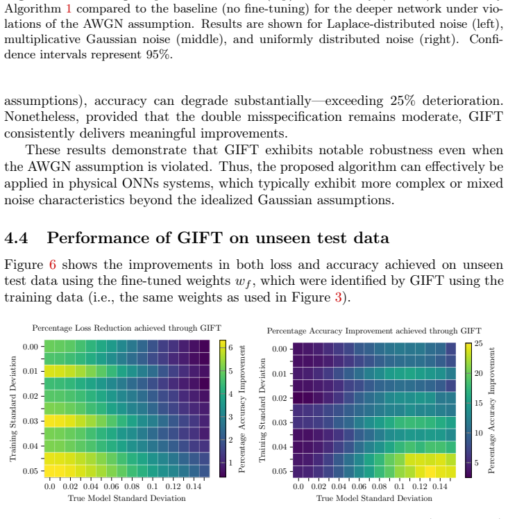
- [Figures 3 and 8] The colorbar labels in the heatmaps are inconsistent: the left panel of Figure 3 says "Percentage Loss Reduction" and the right panel "Percentage Accuracy Improvement", but the colorbar tick labels in some panels omit the percent sign. Please add "%" for clarity.
- [Section 5, conclusion] The sentence "ex situ-trained ONNs" should likely read "in silico-trained ONNs" for consistency with the terminology used throughout the paper. Also, "usefullness" is a typo for "usefulness".
- [Section 2.1, Eq. (15)] The notation for the noise-level parameter s is used both as a subscript in the density φ_s and as a variable in the covariance matrix s^2 I; this is acceptable but should be clearly introduced. More importantly, the subscripts d_i in Eq. (15) are later referred to as d_f(α) without an explicit definition; please clarify the mapping.
Circularity Check
No circularity: GIFT's guarantee is evaluated against the true objective J_st and its descent direction is derived from the noise model, not fitted to the target result.
full rationale
The derivation chain is not circular. The central quantity D[0] (Eqs. 6-7) is an in silico estimator of the derivative of the training gradient with respect to the assumed noise level s0; it is computed from the model M_s, not from the true objective J_st. Algorithm 1 then evaluates candidate weights on the physical ONN via Eval (Eq. 8), which approximates J_st by averaging over true-system outputs, so the selection that yields Theorem 2 is an evaluation against the target objective, not a fit of the target objective back into the direction. Theorem 1's step is a Taylor expansion around w0 using the stationarity of w0 for J_s0 and condition (4); it does not define the conclusion into the assumptions. The cited prior work by the same authors ([30], [54], [52]) supplies the layered AWGN model, proof technique, and conceptual inspiration, respectively, but the model is restated in Eqs. (15)-(18), the stochastic-approximation proofs are reproduced in Appendices A.2-A.3 with reliance on the external textbook [31], and Theorem 2 does not invoke a uniqueness theorem from those papers. The known mathematical fault in Lemma 3 (Eq. 101 gives s^{-2}n^T n - d instead of s^{-1}(s^{-2}n^T n - d)) is a correctness issue in the printed proof of Lemma 2, not a circular reduction: the resulting D[0] is a positive scalar multiple of the intended direction, and because Algorithm 1 tests both ±eta D[0] and selects by true-objective evaluation, the structural logic of the argument is not self-referential. The self-citations are therefore not load-bearing in the circularity sense, and no fitted parameter is renamed as a prediction.
Assumptions & free parameters
free parameters (3)
- s0 =
user-selected estimate of true noise st
- eta
- K1, K2
assumptions (5)
- domain assumption The physical ONN output is described by Ms(x,w,N) with additive white Gaussian noise of true level st.
- standard math Activation function sigma is twice continuously differentiable with polynomially bounded derivatives (C^2_PB).
- ad hoc to paper Condition (4) in Theorem 1 holds.
- domain assumption Data distribution mu has finite moments up to order four (Item A2).
- ad hoc to paper Lemma 3, the formula for the derivative of a product of Gaussian densities, is correct.
Cite this review
Pith. "Pith review of In situ fine-tuning of in silico trained Optical Neural Networks." pith.science (2026). https://pith.science/paper/UGLM7LYK
@misc{pith2026250622122,
  author       = {Pith},
  title        = {Pith review of: In situ fine-tuning of in silico trained Optical Neural Networks},
  year         = {2026},
  howpublished = {\url{https://pith.science/paper/UGLM7LYK}},
  note         = {Machine review of arXiv:2506.22122}
}
abstract
Optical Neural Networks (ONNs) promise significant advantages over traditional electronic neural networks, including ultrafast computation, high bandwidth, and low energy consumption, by leveraging the intrinsic capabilities of photonics. However, training ONNs poses unique challenges, notably the reliance on simplified in silico models whose trained parameters must subsequently be mapped to physical hardware. This process often introduces inaccuracies due to discrepancies between the idealized digital model and the physical ONN implementation, particularly stemming from noise and fabrication imperfections. In this paper, we analyze how noise misspecification during in silico training impacts ONN performance and we introduce Gradient-Informed Fine-Tuning (GIFT), a lightweight algorithm designed to mitigate this performance degradation. GIFT uses gradient information derived from the noise structure of the ONN to adapt pretrained parameters directly in situ, without requiring expensive retraining or complex experimental setups. GIFT comes with formal conditions under which it improves ONN performance. We also demonstrate the effectiveness of GIFT via simulation on a five-layer feed forward ONN trained on the MNIST digit classification task. GIFT achieves up to $28\%$ relative accuracy improvement compared to the baseline performance under noise misspecification, without resorting to costly retraining. Overall, GIFT provides a practical solution for bridging the gap between simplified digital models and real-world ONN implementations.
Figures


Figures from the paper (5 more)




Reference graph
Works this paper leans on
-
[1]
R. Archana and P. S. Eliahim Jeevaraj. Deep learning models for digital image processing: a review. Artificial Intelligence Review, 57(1), 2024
work page 2024
-
[2]
F. Ashtiani, A. J. Geers, and F. Aflatouni. An on-chip photonic deep neural network for image classification.Nature, 606(7914):501–506, 2022
work page 2022
- [3]
-
[4]
L. Cao. AI in Finance: Challenges, Techniques, and Opportunities. ACM Comput. Surv., 55(3), 2022
work page 2022
-
[5]
I. Chakraborty, G. Saha, and K. Roy. Photonic in-memory computing primitive for spiking neural networks using phase-change materials.Phys. Rev. Appl., 11:014063, 2019
work page 2019
-
[6]
Y. Chen, M. Nazhamaiti, H. Xu, Y. Meng, T. Zhou, G. Li, J. Fan, Q. Wei, J. Wu, F. Qiao, L. Fang, and Q. Dai. All-analog photoelectronic chip for high-speed vision tasks.Nature, 623(7985):48–57, 2023
work page 2023
-
[7]
Sili- conphotonicscodesignfordeeplearning
Q.Cheng, J.Kwon, M.Glick, M.Bahadori, L.P.Carloni, andK.Bergman. Sili- conphotonicscodesignfordeeplearning. Proceedings of the IEEE,108(8):1261– 1282, 2020
work page 2020
-
[8]
W.R. Clements, P.C. Humphreys, B.J. Metcalf, W.S. Kolthammer, and I.A. Walmsley. Optimal design for universal multiport interferometers. Optica, 3(12):1460–1465, 2016. 21
work page 2016
Show all 77 references
-
[9]
Dakalbab, M
F. Dakalbab, M. A. Talib, Q. Nasir, and T. Saroufil. Artificial intelligence techniques in financial trading: A systematic literature review. Journal of King Saud University - Computer and Information Sciences, 36(3), 2024
2024
-
[10]
T. F. de Lima, A. N. Tait, H. Saeidi, M. A. Nahmias, H.-T. Peng, S. Abbaslou, B. J. Shastri, and P. R. Prucnal. Noise analysis of photonic modulator neurons. IEEE Journal of Selected Topics in Quantum Electronics, 26(1):1–9, 2020
2020
-
[11]
De Marinis, N
L. De Marinis, N. Andriolli, and G. Contestabile. Analysis of integration tech- nologies for high-speed analog neuromorphic photonics.IEEE Journal of Se- lected Topics in Quantum Electronics, 29(6: Photonic Signal Processing):1–9, 2023
2023
-
[12]
Essiambre, G
R.-J. Essiambre, G. Kramer, P. J. Winzer, G. J. Foschini, and B. Goebel. Capacity limits of optical fiber networks. Journal of Lightwave Technology, 28(4):662–701, 2010
2010
-
[13]
Feldmann, N
J. Feldmann, N. Youngblood, M. Karpov, H. Gehring, X. Li, M. Stappers, M. Le Gallo, X. Fu, A. Lukashchuk, A.S. Raja, T.J. Kippenberg, W.H.P. Per- nice, and H. Bhaskaran. Parallel convolutional processing using an integrated photonic tensor core.Nature, 589(7840):52–58, 2021
2021
-
[14]
Feldmann, N
J. Feldmann, N. Youngblood, C. D. Wright, H. Bhaskaran, and W. H. P. Per- nice. All-optical spiking neurosynaptic networks with self-learning capabilities. Nature, 569(7755):208–214, 2019
2019
-
[15]
C. Feng, J. Gu, H. Zhu, Z. Ying, Z. Zhao, D. Z. Pan, and R. T. Chen. A compact butterfly-style silicon photonic–electronic neural chip for hardware- efficient deep learning.ACS Photonics, 9(12):3906–3916, 2022
2022
-
[16]
Fldzhyan, M.Y
S.A. Fldzhyan, M.Y. Saygin, and S.P. Kulik. Optimal design of error-tolerant reprogrammable multiport interferometers. Optics Letters, 45(9):2632–2635, 2020
2020
-
[17]
Goodfellow, Y
I. Goodfellow, Y. Bengio, and A. Courville.Deep Learning. MIT Press, 2016. http://www.deeplearningbook.org
2016
-
[18]
J. Gu, Z. Zhao, C. Feng, M. Liu, R. T. Chen, and D. Z. Pan. Towards area- efficient optical neural networks: an FFT-based architecture. In2020 25th Asia and South Pacific Design Automation Conference (ASP-DAC), pages 476–481. IEEE, 2020
2020
-
[19]
J. Gu, Z. Zhao, C. Feng, Z. Ying, R. T. Chen, and D. Z. Pan. O2NN: Optical Neural Networks with Differential Detection-Enabled Optical Operands. In 2021 Design, Automation & Test in Europe Conference & Exhibition (DATE), pages 1062–1067, 2021
2021
-
[20]
J. Gu, Z. Zhao, C. Feng, H. Zhu, R. T. Chen, and D. Z. Pan. ROQ: A Noise- Aware Quantization Scheme Towards Robust Optical Neural Networks with Low-bit Controls. In 2020 Design, Automation & Test in Europe Conference & Exhibition (DATE), pages 1586–1589, 2020
2020
-
[21]
J. Gu, H. Zhu, C. Feng, Z. Jiang, M. Liu, S. Zhang, R. T. Chen, and D. Z. Pan. ADEPT: automatic differentiable DEsign of photonic tensor cores. InProceed- ings of the 59th ACM/IEEE Design Automation Conference, DAC ’22, page 937–942, New York, NY, USA, 2022. Association for Co...
2022
-
[22]
Henighan, J
T. Henighan, J. Kaplan, M. Katz, M. Chen, C. Hesse, J. Jackson, H. Jun, T. B. Brown, P. Dhariwal, S. Gray, C. Hallacy, B. Mann, A. Radford, A. Ramesh, N. Ryder, D. M. Ziegler, J. Schulman, D. Amodei, and S. McCandlish. Scaling laws for autoregressive generative modeling.arXiv ...
2010 arXiv
-
[23]
Hestness, S
J. Hestness, S. Narang, N. Ardalani, G. Diamos, H. Jun, H. Kianinejad, M. M. A. Patwary, Y. Yang, and Y. Zhou. Deep learning scaling is predictable, empirically. arXiv preprint arXiv:1712.00409, 2017
2017 arXiv
-
[24]
Kaplan, S
J. Kaplan, S. McCandlish, T. Henighan, T. B. Brown, B. Chess, R. Child, S. Gray, A. Radford, J. Wu, and D. Amodei. Scaling laws for neural language models. arXiv preprint arXiv:2001.08361, 2020
2001 arXiv
-
[25]
Kirtas, A
M. Kirtas, A. Oikonomou, N. Passalis, G. Mourgias-Alexandris, M. Moralis- Pegios, N. Pleros, and A. Tefas. Quantization-aware training for low precision photonic neural networks.Neural Networks, 155:561–573, 2022
2022
-
[26]
Kirtas, N
M. Kirtas, N. Passalis, G. Mourgias-Alexandris, G. Dabos, N. Pleros, and A. Tefas. Learning photonic neural network initialization for noise-aware end- to-end fiber transmission. In2022 30th European Signal Processing Conference (EUSIPCO), pages 1731–1735, 2022
2022
-
[27]
Kirtas, N
M. Kirtas, N. Passalis, G. Mourgias-Alexandris, G. Dabos, N. Pleros, and A. Tefas. Robust architecture-agnostic and noise resilient training of photonic deep learning models. IEEE Transactions on Emerging Topics in Computa- tional Intelligence, 7(1):140–149, 2023
2023
-
[28]
Kosmella, M
G. Kosmella, M. G. de Queiroz, M. Hejda, W. Peelaers, and T. Van Vaeren- bergh. Towards a noise-robust automated search of photonic circuit designs. In IEEE Photonics Benelux Chapter Annual Symposium 2024, 2024
2024
-
[29]
Kosmella, J
G. Kosmella, J. Sanders, B. Shi, and R. Stabile. Higher-accuracy photonic neu- ral networks via duplication schemes for noise reduction. In2023 International Conference on Photonics in Switching and Computing (PSC), pages 1–4, 2023
2023
-
[30]
Kosmella, R
G. Kosmella, R. Stabile, and J. Sanders. Noise-resilient designs and analy- sis for optical neural networks. Neuromorphic Computing and Engineering, 4(4):044002, 2024
2024
-
[31]
Kushner and G
H. Kushner and G. Yin.Stochastic Approximation and Recursive Algorithms and Applications. Springer Science & Business Media, 2003
2003
-
[32]
X. Li, R. Mardling, and J. Armstrong. Channel capacity of im/dd optical com- munication systems and of aco-ofdm. In2007 IEEE International Conference on Communications, pages 2128–2133, 2007
2007
-
[33]
Y. Li. Deep reinforcement learning: An overview. arXiv preprint arXiv:1701.07274, 2018
2018 arXiv
-
[34]
A. E.-J. Lim, J. Song, Q. Fang, C. Li, X. Tu, N. Duan, K. K. Chen, R. P.- C. Tern, and T.-Y. Liow. Review of silicon photonics foundry efforts.IEEE Journal of Selected Topics in Quantum Electronics, 20(4):405–416, 2014
2014
-
[35]
P. Y. Ma, A. N. Tait, T. F. de Lima, C. Huang, B. J. Shastri, and P. R. Prucnal. Photonic independent component analysis using an on-chip microring weight bank. Opt. Express, 28(2):1827–1844, 2020. 23
2020
-
[36]
Marchesin, M
F. Marchesin, M. Hejda, T. Melendez Carmona, S. Di Carlo, A. Savino, F. Pa- vanello, T. Van Vaerenbergh, and P. Bienstman. Braided interferometer mesh for robust photonic matrix-vector multiplications with non-ideal components. Optics Express, 33(2):2227–2246, 2025
2025
-
[37]
P. L. McMahon. The physics of optical computing.Nature Reviews Physics, 5(12):717–734, 2023
2023
-
[38]
X. Meng, G. Zhang, N. Shi, G. Li, J. Azaña, J. Capmany, J. Yao, Y. Shen, W. Li, N. Zhu, and M. Li. Compact optical convolution processing unit based on multimode interference.Nature Communications, 14(1):3000, 2023
2023
-
[39]
Mennella, U
C. Mennella, U. Maniscalco, G. De Pietro, and M. Esposito. Ethical and regu- latory challenges of ai technologies in healthcare: A narrative review.Heliyon, 10(4), 2024
2024
-
[40]
Mirza, F
A. Mirza, F. Sunny, P. Walsh, K. Hassan, S. Pasricha, and M. Nikdast. Sili- con photonic microring resonators: A comprehensive design-space exploration and optimization under fabrication-process variations.IEEE Transactions on Computer-Aided Design of Integrated Circuits and S...
2022
-
[41]
Miscuglio and V
M. Miscuglio and V. J. Sorger. Photonic tensor cores for machine learning. Applied Physics Reviews, 2020
2020
-
[42]
Mourgias-Alexandris, M
G. Mourgias-Alexandris, M. Moralis-Pegios, A. Tsakyridis, S. Simos, G. Dabos, A. Totovic, N. Passalis, M. Kirtas, T. Rutirawut, F. Y. Gardes, A. Tefas, and N. Pleros. Noise-resilient and high-speed deep learning with coherent silicon photonics. Nature Communications, 13(1):5572, 2022
2022
-
[43]
Mourgias-Alexandris, A
G. Mourgias-Alexandris, A. Tsakyridis, N. Passalis, A. Tefas, K. Vyrsokinos, and N. Pleros. An all-optical neuron with sigmoid activation function.Opt. Express, 27(7):9620–9630, 2019
2019
-
[44]
S. Ning, H. Zhu, C. Feng, J. Gu, Z. Jiang, Z. Ying, J. Midkiff, S. Jain, M. H. Hlaing, D. Z. Pan, and R. T. Chen. Photonic-electronic integrated circuits for high-performance computing and ai accelerators. Journal of Lightwave Technology, 42(22):7834–7859, 2024
2024
-
[45]
Oikonomou, M
A. Oikonomou, M. Kirtas, N. Passalis, G. Mourgias-Alexandris, M. Moralis- Pegios, N. Pleros, and A. Tefas. A robust, quantization-aware training method for photonic neural networks. InEngineering Applications of Neural Networks, pages 427–438, Cham, 2022. Springer Internationa...
2022
-
[46]
D. W. Otter, J. R. Medina, and J. K. Kalita. A survey of the usages of deep learning for natural language processing.IEEE Transactions on Neural Networks and Learning Systems, 32(2):604–624, 2021
2021
-
[47]
Passalis, M
N. Passalis, M. Kirtas, G. Mourgias-Alexandris, G. Dabos, N. Pleros, and A. Tefas. Training noise-resilient recurrent photonic networks for financial time series analysis. In2020 28th European Signal Processing Conference (EU- SIPCO), pages 1556–1560, 2021
2021
-
[48]
Passalis, G
N. Passalis, G. Mourgias-Alexandris, N. Pleros, and A. Tefas. Initializing pho- tonic feed-forward neural networks using auxiliary tasks. Neural Networks, 129:103–108, 2020. 24
2020
-
[49]
Passalis, G
N. Passalis, G. Mourgias-Alexandris, A. Tsakyridis, N. Pleros, and A. Tefas. Training deep photonic convolutional neural networks with sinusoidal activa- tions. IEEE Transactions on Emerging Topics in Computational Intelligence, 5(3):384–393, 2021
2021
-
[50]
M. Reda, A. Onsy, A. Y. Haikal, and A. Ghanbari. Path planning algorithms in the autonomous driving system: A comprehensive review. Robotics and Autonomous Systems, 174:104630, 2024
2024
-
[51]
Aconstructivepredic- tion of the generalization error across scales.arXiv preprint arXiv:1909.12673, 2019
J.S.Rosenfeld, A.Rosenfeld, Y.Belinkov, andN.Shavit. Aconstructivepredic- tion of the generalization error across scales.arXiv preprint arXiv:1909.12673, 2019
1909 arXiv
-
[52]
Sanders, S.C
J. Sanders, S.C. Borst, A.J.E.M. Janssen, and J.S.H. van Leeuwaarden. Op- timality gaps in asymptotic dimensioning of many-server systems.Operations Research Letters, 44(3):359–365, 2016
2016
-
[53]
Semenova, L
N. Semenova, L. Larger, and D. Brunner. Understanding and mitigating noise in trained deep neural networks.Neural Networks, 146:151–160, 2022
2022
-
[54]
Senen-Cerda and J
A. Senen-Cerda and J. Sanders. Almost sure convergence of dropout algorithms for neural networks.arXiv preprint arXiv:2002.02247, 2023
2002 arXiv
-
[55]
B. J. Shastri, A. N. Tait, T. Ferreira de Lima, W. H. P. Pernice, H. Bhaskaran, C. D. Wright, and P. R. Prucnal. Photonics for artificial intelligence and neuromorphic computing. Nature Photonics, 15(2):102–114, 2021
2021
-
[56]
Y. Shen, N. C. Harris, S. Skirlo, M. Prabhu, T. Baehr-Jones, M. Hochberg, X. Sun, S. Zhao, H. Larochelle, D. Englund, and M. Soljačić. Deep learning with coherent nanophotonic circuits.Nature Photonics, 11(7):441–446, 2017
2017
-
[57]
B. Shi, N. Calabretta, and R. Stabile. First demonstration of a two-layer all- optical neural network by using photonic integrated chips and soas. In45th European Conference on Optical Communication (ECOC 2019). IET, 2019
2019
-
[58]
B. Shi, N. Calabretta, and R. Stabile. Deep neural network through an inp soa-based photonic integrated cross-connect.IEEE Journal of Selected Topics in Quantum Electronics, 26(1):1–11, 2020
2020
-
[59]
B. Shi, B. Pan, N. Calabretta, and R. Stabile. Noise analysis of soa-based all-optical photonic deep neural network with wdm input. In Photonics in Switching and Computing 2021. Optica Publishing Group, 2021
2021
-
[60]
Y. Shi, S. Xiang, X. Guo, Y. Zhang, H. Wang, D. Zheng, Y. Zhang, Y. Han, Y. Zhao, X. Zhu, X. Chen, X. Li, and Y. Hao. Photonic integrated spik- ing neuron chip based on a self-pulsating dfb laser with a saturable absorber. Photonics Research, 11(8):1382–1389, 2023
2023
-
[61]
Sludds, S
A. Sludds, S. Bandyopadhyay, Z. Chen, Z. Zhong, J. Cochrane, L. Bernstein, D. Bunandar, P. B. Dixon, S. A. Hamilton, M. Streshinsky, A. N., T. Baehr- Jones, M. Hochberg, M. Ghobadi, R. Hamerly, and D. Englund. Delocalized photonic deep learning on the internet’s edge. Science,...
2022
-
[62]
Spall, X
J. Spall, X. Guo, and A. I. Lvovsky. Hybrid training of optical neural networks. Optica, 9(7):803–811, 2022. 25
2022
-
[63]
Sunny, A
F. Sunny, A. Mirza, M. Nikdast, and S. Pasricha. Crosslight: A cross-layer op- timized silicon photonic neural network accelerator. In2021 58th ACM/IEEE Design Automation Conference (DAC), pages 1069–1074, 2021
2021
-
[64]
A. N. Tait, T. F. de Lima, E. Zhou, A. X. Wu, M. A. Nahmias, B. J. Shastri, and P. R. Prucnal. Neuromorphic photonic networks using silicon photonic weight banks.Scientific Reports, 7(1):7430, 2017
2017
-
[65]
A.N. Tait, T. Ferreira de Lima, M.A. Nahmias, H.B. Miller, H.-T. Peng, B.J. Shastri, and P.R. Prucnal. Silicon photonic modulator neuron.Physical Review Applied, 11(6):064043, 2019
2019
-
[66]
Varri, F
A. Varri, F. Brückerhoff-Plückelmann, J. Dijkstra, D. Wendland, R. Bankwitz, A. Agnihotri, and W. H. P. Pernice. Noise-resilient photonic analog neural networks. J. Lightwave Technol., 42(22):7969–7976, 2024
2024
-
[67]
H. Wang, T. Fu, Y. Du, W. Gao, K. Huang, Z. Liu, P. Chandak, S. Liu, P. Van Katwyk, A. Deac, A. Anandkumar, K. Bergen, C. P. Gomes, S. Ho, P. Kohli, J. Lasenby, J. Leskovec, T.-Y. Liu, A. Manrai, D. Marks, B. Ram- sundar, L. Song, J. Sun, J. Tang, P. Veličković, M. Welling, L....
2023
-
[68]
Z. Wang, L. Chang, F. Wang, T. Li, and T. Gu. Integrated photonic metasys- tem for image classifications at telecommunication wavelength.Nature Com- munications, 13(1):2131, 2022
2022
-
[69]
L. G. Wright, T. Onodera, M. M. Stein, T. Wang, D. T. Schachter, Z. Hu, and P. L. McMahon. Deep physical neural networks trained with backpropagation. Nature, 601(7894):549–555, 2022
2022
-
[70]
T. Xu, W. Zhang, J. Zhang, Z. Luo, Q. Xiao, B. Wang, M. Luo, X. Xu, B. J. Shastri, P. R. Prucnal, and C. Huang. Control-free and efficient integrated photonic neural networks via hardware-aware training and pruning.Optica, 11(8):1039–1049, 2024
2024
-
[71]
X. Xu, M. Tan, B. Corcoran, J. Wu, A. Boes, T. G. Nguyen, S. T. Chu, B. E. Little, D. G. Hicks, R. Morandotti, A. Mitchell, and D. J. Moss. 11 tops photonic convolutional accelerator for optical neural networks.Nature, 589(7840):44–51, 2021
2021
-
[72]
Y. Zhan, H. Zhang, H. Lin, L. K. Chin, H. Cai, M. Faeyz Karim, D. P. Poenar, X. Jiang, M.-W. Mak, L. C. Kwek, and A. Q. Liu. Physics-aware analytic- gradient training of photonic neural networks. Laser & Photonics Reviews, 18(4):2300445, 2024
2024
-
[73]
Z. Zhao, J. Gu, Z. Ying, C. Feng, R. T. Chen, and D. Z. Pan. Design technology for scalable and robust photonic integrated circuits: Invited paper. In2019 IEEE/ACM International Conference on Computer-Aided Design (ICCAD), pages 1–7, 2019
2019
-
[74]
T. Zhou, X. Lin, J. Wu, Y. Chen, H. Xie, Y. Li, J. Fan, H. Wu, L. Fang, and Q. Dai. Large-scale neuromorphic optoelectronic computing with a reconfig- urable diffractive processing unit.Nature Photonics, 15(5):367–373, 2021
2021
-
[75]
H. Zhu, J. Gu, C. Feng, M. Liu, Z. Jiang, R. T. Chen, and D. Z. Pan. ELight: Enabling Efficient Photonic In-Memory Neurocomputing with Life Enhance- ment. In 2022 27th Asia and South Pacific Design Automation Conference (ASP-DAC), pages 332–338, 2022. 26
2022
-
[76]
Y. Zhu, M. Liu, L. Xu, L. Wang, X. Xiao, and S. Yu. Multi-wavelength parallel training and quantization-aware tuning for wdm-based optical convolutional neural networks considering wavelength-relative deviations. InProceedings of the 28th Asia and South Pacific Design Automati...
2023
-
[77]
X α∈Si s−2 0 N α,{mk} T N α,{mk} − df (α) R(ℓ),{k} A(ℓ−1),{k} T # jk ; (123) and similarly, for eachjth component of theℓth bias vector, fb(ℓ) j ((X {k}, Y{k}), N{mk}) =
(120) Since both terms in the right-hand side of (115) converge almost surely, Shi a.s. − − − − − − − → K1,K2→∞ E[f (A, B)]. (121) That is it. □ 34 A.7 Proof of Lemma 2 We prove Lemma 2 via Lemma 4. This requires verifying that the conditions of Lemma 4 hold for D[0] W (ℓ) (K1...
Reviewed August 6, 2026 · model on record in the stance chip above.
Discussion (0). Continue with ORCID to comment.