REVIEW 3 major objections 6 minor 54 references
Magnetohydrodynamic waves in braided magnetic fields
T0 review · 3 major / 6 minor · reviewed 2026-08-14 · deepseek-v4-flash
Pith's one-line read This paper claims that in a braided coronal magnetic field, phase mixing spreads wave-energy dissipation across the entire magnetic structure rather than confining it to density-gradient boundaries.
desk verdict Solid simulation study of phase mixing in braided fields; the qualitative volume-filling claim holds, but the 'larger cross-section for dissipation' is inferred from vorticity, not directly measured, and the quantitative heating enhancement is modest and resolution-sensitive. read the letter →
The pith
A machine-rendered reading of the paper's core claim, the machinery that carries it, and where it could break.
The reading
What carries the argument
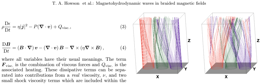
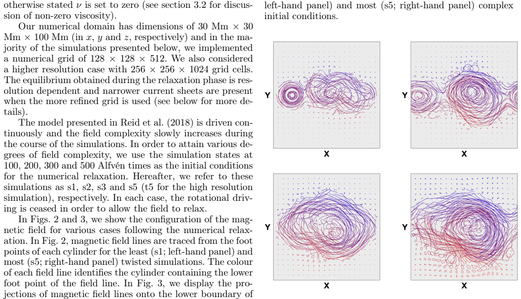
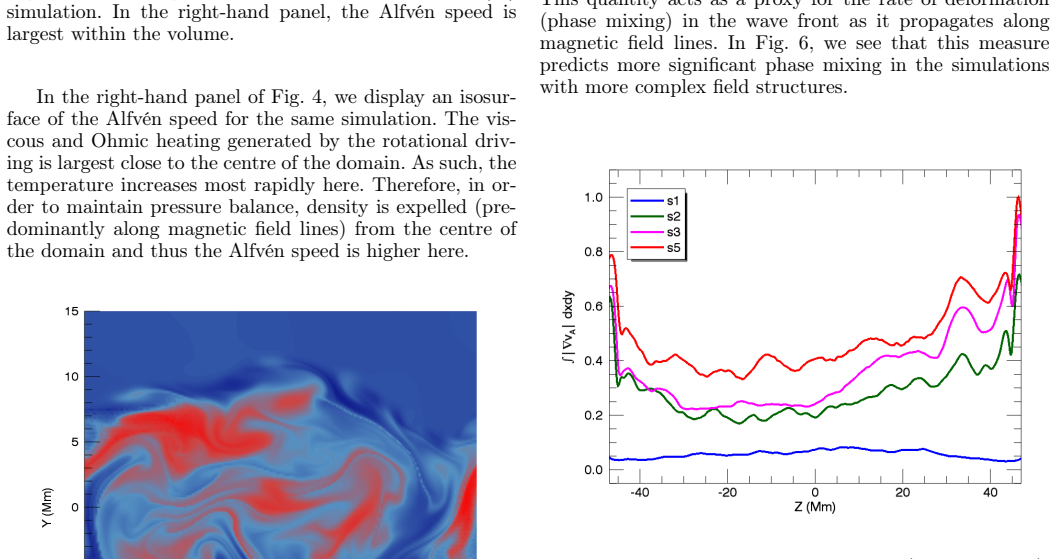
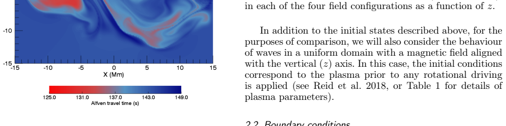
The argument is carried by three related objects: the Alfvén travel time $\Omega(x,y)=\int ds/v_A$ along each magnetic field line, whose spatial gradients set where and how fast phase mixing creates small scales; the background current sheets, whose strong vertical currents interact with the wave's perturbed horizontal field to rotate the wave's polarization; and the volume-integrated vorticity $\int|\omega|\,dV$, used as a proxy for small-scale formation and hence viscous dissipation. The braided equilibria themselves are produced by relaxing a stressed, continuously driven magnetic field into a numerical equilibrium, so all wave dynamics are studied against an inhomogeneous background rather than a prescribed density profile.
What would settle it
A decisive test is a resolution study: run the same wave driver through a braided equilibrium whose background current sheets are resolved at the true dissipation scale and compare the volume-integrated vorticity and viscous heating with the uniform-field case; if the enhanced, volume-filling dissipation disappears once the sheets are resolved, or if it persists when the sheets are artificially smoothed away, the claimed mechanism would be refuted or confirmed accordingly.
Extended reading notes
Core claim
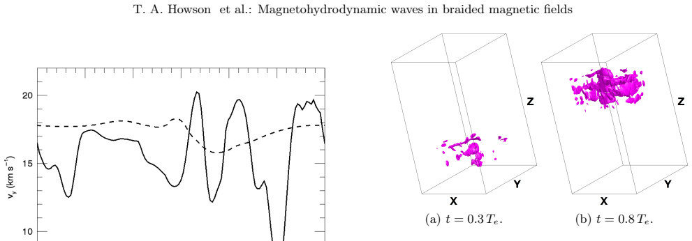
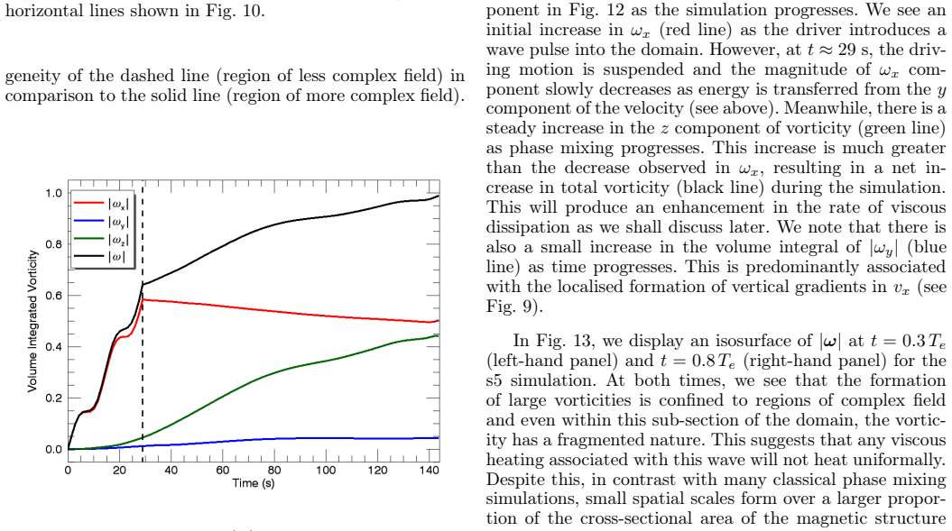
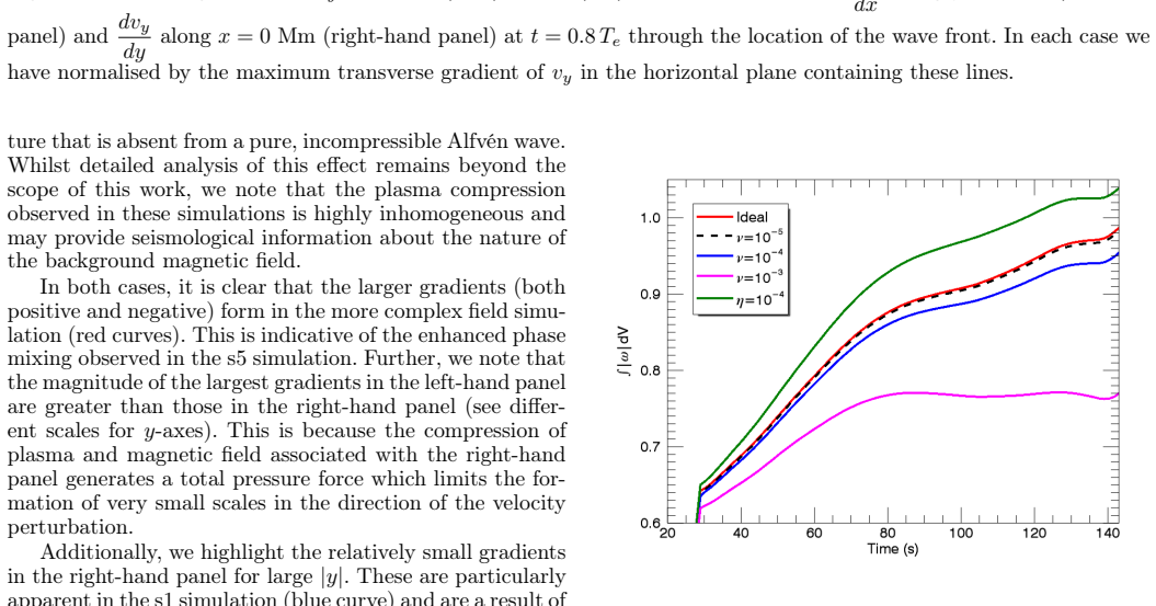
The central discovery is that phase mixing in a braided magnetic field is volume-filling rather than boundary-localized. In classical phase mixing, a density gradient across a loop creates a narrow layer of small scales; here, the braided field's spatially distributed gradients in Alfvén speed and varying field-line lengths create small transverse gradients across the whole wave front. In addition, the strong vertical currents of the background field interact with the wave's perturbed horizontal field to generate a Lorentz force that locally transfers energy between the two horizontal velocity components, modifying the wave's polarization. The simulations show that volume-integrated vorticity grows with field complexity, and that viscous heating in the most braided case is more than twice the uniform-field case at Reynolds number $10^3$, with a larger relative enhancement at lower viscosity. Because the dissipated energy is spread over the whole braided cross-section, the paper concludes that the standard objection that phase mixing cannot sustain the observed corona does not apply in this regime.
Load-bearing premise
The simulations' braided magnetic equilibria have current sheets whose width is limited by the numerical grid, and the paper itself notes that higher resolution produces narrower sheets; if real coronal sheets are much narrower, the quantitative heating enhancement could change, though the volume-filling phase mixing would probably survive.
Editorial extensions
If this is right
- Wave-energy dissipation in a non-ideal plasma is no longer confined to narrow boundary layers, so phase mixing remains viable as a coronal heating mechanism even under the constraints raised for classical models.
- The rate at which small scales form, and hence the heating rate, increases with the complexity of the background field; more braided equilibria dissipate more of the same injected wave energy.
- Small spatial gradients in the driving motions at the footpoints are amplified into large gradients in the corona, so even smooth, large-scale photospheric driving can produce strong phase mixing.
- The wave's weak compressibility and its phase-mixing pattern carry information about the background field, potentially allowing coronal seismology to probe magnetic complexity.
- With continuous driving, the wide range of field-line lengths and Alfvén speeds should make it easy to excite resonances, so continuous drivers would deposit more energy than the single pulses studied here.
Reading between the lines
- Going beyond the paper: the same volume-filling phase mixing should make wave heating self-limiting in a real corona, because the heating smoothes the very Alfvén-speed gradients that create the small scales; the simulations stop before such feedback develops.
- Going beyond the paper: if real coronal current sheets are systematically narrower than the grid can resolve, the dissipation enhancement at true coronal Reynolds numbers is likely larger than simulated, making the reported heating ratios lower bounds rather than converged estimates.
- Going beyond the paper: polarization rotation by background currents implies that observations of a single transverse velocity component could misclassify a wave mode; synthetic observables from these runs could calibrate that bias.
Signed reviews
Editorial analysis
A structured set of objections, weighed in public.
Referee Report
Summary. This paper investigates the propagation of a small-amplitude transverse MHD wave pulse through three-dimensional braided magnetic fields, using simulations initialised from the stress-twisted equilibria of Reid et al. (2018). Four braided configurations of increasing complexity (s1, s2, s3, s5) and a uniform-field baseline are driven with a single-period sinusoid on the lower boundary. The authors analyze wave-front deformation, phase mixing, polarization changes, and viscous dissipation. They conclude that phase mixing is volume-filling in braided fields, that wave energy is deposited over a larger cross-sectional area than in classical phase-mixing models, and that the rate of small-scale formation increases with field complexity.
Significance. If confirmed, the volume-filling phase-mixing picture is an important departure from the classical idea that phase mixing occurs only at density-gradient boundaries. The simulations are physically motivated, use a standard and well-tested code (Lare3D), include a resolution study (s5 vs. t5), and provide a quantitative proxy for field complexity (I(z)). The diagnostics are internally consistent, and the authors are appropriately cautious about the small energy budget and the need for continuous driving in future work. However, the headline claim about the spatial distribution of dissipation is not directly measured, and the quantitative complexity dependence is resolution-sensitive.
major comments (3)
- [§3.3, Figs. 18 and 19] The central claim that wave energy is dissipated over a larger cross-section in braided fields is not directly supported by the dissipation diagnostics presented. The paper reports volume-integrated |ω| (Fig. 18) and cumulative volume-integrated viscous heating (Fig. 19), but the only spatial maps shown (Fig. 13) are isosurfaces of |ω|, not of the viscous heating rate Q_visc. Since Q_visc depends on the symmetric rate-of-strain tensor rather than the antisymmetric vorticity, the spatial distribution of |ω| is not a direct proxy for the location of viscous heating. The authors should either (i) compute and display maps or cross-sections of the actual viscous heating rate (or the rate-of-strain magnitude) to substantiate the "greater cross-section" claim, or (ii) explicitly restrict the claim to the vorticity field and soften the dissipation statement.
- [§3.4, Fig. 20 and §2.1] The quantitative claim that the small-scale formation rate is a function of field complexity is not numerically converged. The paper acknowledges in Section 2.1 that the relaxed equilibria are resolution dependent ("narrower current sheets are present when the more refined grid is used"), and Fig. 20 shows that the t5 simulation produces systematically higher volume-integrated |ω| than the corresponding s5 run. Thus the differences between s1, s2, s3, and s5 are at least partly attributable to how the grid resolves the current sheets, not solely to the intended field complexity. The qualitative ordering may be robust, but the specific quantitative statements (e.g., the factor-of-two heating enhancement in Fig. 19, and the resolution-normalized vorticity curves) are not. The authors should either demonstrate a convergence trend (e.g., show that s5 and t5 bracket the converged result) or temper the quantitative claims.
- [Abstract and §4] The abstract and Section 4 assert that wave energy is deposited "over a larger cross-section than in classical phase mixing models." However, the simulations do not include a classical phase-mixing configuration as a baseline; the only comparison is to a uniform-field case. Since classical phase mixing proceeds from a transverse Alfvén speed gradient (e.g., a density-enhanced loop), the comparison in the present study is indirect. The authors should either include a simple classical phase-mixing run with the same driver and energy budget, or explicitly state that the "greater cross-section" claim is relative to a uniform background and is an inference from the spatial extent of the vorticity gradients.
minor comments (6)
- [§3.4] Typo: "intoduced" should be "introduced".
- [§3.3, Fig. 19 caption] Typo: "obseverd" should be "observed".
- [§4] Typo: "identied" should be "identified".
- [§3.5] Typo: "horiztontal" should be "horizontal".
- [§2.1] Typo: "caclulate" should be "calculate".
- [References] The reference "Goossens, M. Erdélyi, R. & Ruderman, M. S. 2011" is missing an ampersand between the authors; it should read "Goossens, M., Erdélyi, R., & Ruderman, M. S. 2011".
Circularity Check
No significant circularity; the central wave-dissipation claims are derived from independent MHD simulations and measured diagnostics.
full rationale
The paper's central claims—volume-filling phase mixing and enhanced viscous dissipation in braided fields—are derived from MHD simulations of an externally imposed wave packet, not from a parameter fitted to the target quantity. The initial braided equilibria are taken from Reid et al. (2018), a self-cited prior simulation, but that work supplies only the background state; it does not contain or assume the wave phase-mixing result, and the wave evolution is simulated independently here. The diagnostics used (vorticity, viscous heating, Alfvén-travel-time maps) are measured from simulation output and are not defined in terms of the conclusions. For example, the claim that wave energy is deposited over a larger cross-section is inferred from distributed small-scale vorticity and from isosurfaces of the vorticity magnitude; whether one agrees with that inference, it is not equivalent to an input by construction. No equation reduces a reported prediction to a fitted parameter, and no load-bearing uniqueness or ansatz is imported via self-citation. The resolution dependence of the initial equilibria is a legitimate quantitative robustness concern, but it is not a circularity.
Assumptions & free parameters
free parameters (5)
- wave driver amplitude v0 =
20 km/s
- wave driver period tau =
30 s
- viscosity coefficients nu =
10^-3, 10^-4, 10^-5
- Gaussian width l of non-uniform driver =
6 Mm
- initial condition times =
100, 200, 300, 500 Alfven times
assumptions (5)
- domain assumption The ideal MHD equations with viscous and Ohmic dissipation describe the coronal plasma (Eqs. 1-4).
- domain assumption The relaxed background field is approximately force-free with beta < 1 and currents dominated by the parallel component.
- domain assumption The braided field states from Reid et al. (2018), after relaxation, are representative of coronal braided magnetic fields.
- domain assumption The relaxation phase leaves the plasma in a numerical equilibrium with negligible background flows relative to the wave amplitude.
- domain assumption The Lare3D code accurately solves the specified MHD equations at the quoted resolution.
Cite this review
Pith. "Pith review of Magnetohydrodynamic waves in braided magnetic fields." pith.science (2026). https://pith.science/paper/ULM2AM2I
@misc{pith2026190803089,
  author       = {Pith},
  title        = {Pith review of: Magnetohydrodynamic waves in braided magnetic fields},
  year         = {2026},
  howpublished = {\url{https://pith.science/paper/ULM2AM2I}},
  note         = {Machine review of arXiv:1908.03089}
}
read the original abstract
We consider a series of MHD simulations in which a small amplitude, transverse velocity perturbation is introduced into a complex magnetic field. We analysed the deformation of the wave fronts as the perturbation propagates through the braided magnetic structures and explore the nature of Alfv\'enic wave phase mixing in this regime. Spatial gradients in the local Alfv\'en speed and variations in the length of magnetic field lines ensure that small scales form throughout the propagating wave front due to phase mixing. Additionally, the presence of complex, intricate current sheets associated with the background field locally modifies the polarisation of the wave front. The combination of these two effects enhances the rate of viscous dissipation, particularly in more complex field configurations. Unlike in classical phase mixing configurations, the greater spatial extent of Alfv\'en speed gradients ensures that wave energy is deposited over a larger cross-section of the magnetic structure. Further, the complexity of the background magnetic field ensures that small gradients in a wave driver can map to large gradients within the coronal plasma. The phase mixing of MHD waves in a complex magnetic field will progress throughout the braided volume. As a result, in a non-ideal regime wave energy will be dissipated over a greater cross-section than in classical phase mixing models. The formation rate of small spatial scales in a propagating wave front is a function of the complexity of the background magnetic field. As such, if the coronal field is sufficiently complex it remains plausible that phase mixing induced wave heating can contribute to maintaining observed temperatures. Furthermore, the weak compressibility of the transverse wave and the observed phase mixing pattern may provide seismological information about the nature of the background plasma.
Figures

Figures from the paper (16 more)





Reference graph
Works this paper leans on
-
[1]
Afanasyev, A. N. & Zhukov, A. N. 2018, A&A, 614, A139
work page 2018
-
[2]
D., Longbottom, A
Arber, T. D., Longbottom, A. W., Gerrard, C. L., & Milne, A. M. 2001, Journal of Computational Physics, 171, 151
2001
-
[3]
2015, Philosophical Transactions of the Royal Society of London Series A, 373, 20140261
Arregui, I. 2015, Philosophical Transactions of the Royal Society of London Series A, 373, 20140261
work page 2015
-
[4]
J., de Pontieu, B., Schrijver, C
Aschwanden, M. J., de Pontieu, B., Schrijver, C. J., & Title, A. M. 2002, Sol. Phys., 206, 99
work page 2002
-
[5]
J., Fletcher, L., Schrijver, C
Aschwanden, M. J., Fletcher, L., Schrijver, C. J., & Alexander, D. 1999, ApJ, 520, 880
1999
-
[6]
J., De Moortel, I., & Kiddie, G
Cargill, P. J., De Moortel, I., & Kiddie, G. 2016, ApJ, 823, 31
work page 2016
-
[7]
Cranmer, S. R. & van Ballegooijen, A. A. 2005, ApJS, 156, 265 De Moortel, I., Ireland, J., & Walsh, R. W. 2000, A&A, 355, L23 Duckenfield, T., Anfinogentov, S. A., Pascoe, D. J., & Nakariakov, V. M. 2018, ApJ, 854, L5
work page 2005
-
[8]
Engvold, O. 2008, in IAU Symposium, Vol. 247, Waves & Oscil- lations in the Solar Atmosphere: Heating and Magneto-Seismology, ed. R. Erdélyi & C. A. Mendoza-Briceno, 152–157 Erdélyi, R. & Ballai, I. 2007, Astronomische Nachrichten, 328, 726
work page 2008
Show all 54 references
-
[9]
Goossens, M., Terradas, J., Andries, J., Arregui, I., & Ballester, J. L. 2009, A&A, 503, 213
2009
-
[10]
2013, ApJ, 768, 191
Goossens, M., Van Doorsselaere, T., Soler, R., & Verth, G. 2013, ApJ, 768, 191
2013
-
[11]
Erdélyi, R
Goossens, M. Erdélyi, R. & Ruderman, M. S. 2011, Space Science Reviews, 158, 289
2011
-
[12]
& Priest, E
Heyvaerts, J. & Priest, E. R. 1983, A&A, 117, 220
1983
-
[13]
J., & Erdélyi, R
Hillier, A., Morton, R. J., & Erdélyi, R. 2013, ApJ, 779, L16
2013
-
[14]
Ionson, J. A. 1978, Astrophys. J., 226, 650
1978
-
[15]
C., Liu, C., Sun, X., et al
Joshi, N. C., Liu, C., Sun, X., et al. 2015, ApJ, 812, 50
2015
-
[16]
& Van Doorsselaere, T
Karampelas, K. & Van Doorsselaere, T. 2018, A&A, 610, L9
2018
-
[17]
Klimchuk, J. A. 2006, Solar Physics, 234, 41
2006
-
[18]
Lazzaro, E., Lontano, M., & Ryutov, D. D. 2000, Phys. Rev. E, 61, 3069
2000
-
[19]
2016, ApJ, 817, 39
Lim, E.-K., Yurchyshyn, V., Park, S.-H., et al. 2016, ApJ, 817, 39
2016
-
[20]
W., Rickard, G
Longbottom, A. W., Rickard, G. J., Craig, I. J. D., & Sneyd, A. D. 1998, ApJ, 500, 471
1998
-
[21]
Longcope, D. W. & Sudan, R. N. 1994, ApJ, 437, 491
1994
-
[22]
2017, Scientific Reports, 7, 14820
Magyar, N., Van Doorsselaere, T., & Goossens, M. 2017, Scientific Reports, 7, 14820
2017
-
[23]
McEwan, M. P. & De Moortel, I. 2006, A&A, 448, 763
2006
-
[24]
W., de Pontieu, B., Carlsson, M., et al
McIntosh, S. W., de Pontieu, B., Carlsson, M., et al. 2011, Nature, 475, 477
2011
-
[25]
McLaughlin, J. A. 2016, Journal of Astrophysics and Astronomy, 37, 2
2016
-
[26]
A., Thurgood, J
McLaughlin, J. A., Thurgood, J. O., Botha, G. J. J., & Wiggs, J. A. 2019, MNRAS, 484, 1390
2019
-
[27]
J., Tomczyk, S., & Pinto, R
Morton, R. J., Tomczyk, S., & Pinto, R. 2015, Nature Communica- tions, 6, 7813
2015
-
[28]
J., Tomczyk, S., & Pinto, R
Morton, R. J., Tomczyk, S., & Pinto, R. F. 2016, ApJ, 828, 89
2016
-
[29]
& Thompson, B
Ofman, L. & Thompson, B. J. 2002, ApJ, 574, 440 O’Hara, J. P. & De Moortel, I. 2016, A&A, 594, A67 Article number, page 13 of 14 A&A proofs: manuscript no. WBF
2002
-
[30]
J., Tsuneta, S., Berger, T
Okamoto, T. J., Tsuneta, S., Berger, T. E., et al. 2007, Science, 318, 1577
2007
-
[31]
& De Moortel, I
Pagano, P. & De Moortel, I. 2017, A&A, 601, A107
2017
-
[32]
Parker, E. N. 1972, Astrophys. J., 174, 499
1972
-
[33]
Parnell, C. E. & De Moortel, I. 2012, Philosophical Transactions of the Royal Society of London Series A, 370, 3217
2012
-
[34]
J., Wright, A
Pascoe, D. J., Wright, A. N., & De Moortel, I. 2010, ApJ, 711, 990
2010
-
[35]
J., Wright, A
Pascoe, D. J., Wright, A. N., & De Moortel, I. 2011, ApJ, 731, 73
2011
-
[36]
V., & Nordlund, Å
Peter, H., Gudiksen, B. V., & Nordlund, Å. 2004, ApJ, 617, L85
2004
-
[37]
I., Candelaresi, S., Russell, A
Pontin, D. I., Candelaresi, S., Russell, A. J. B., & Hornig, G. 2016, Plasma Physics and Controlled Fusion, 58, 054008
2016
-
[38]
Prokopyszyn, A. P. K., Hood, A. W., & De Moortel, I. 2019, A&A
2019
-
[39]
2016, ApJ, 830, 21
Reale, F., Orlando, S., Guarrasi, M., et al. 2016, ApJ, 830, 21
2016
-
[40]
W., Parnell, C
Reid, J., Hood, A. W., Parnell, C. E., Browning, P. K., & Cargill, P. J. 2018, A&A, 615, A84
2018
-
[41]
Similon, P. L. & Sudan, R. N. 1989, ApJ, 336, 442
1989
-
[42]
K., Zaqarashvili, T
Srivastava, A. K., Zaqarashvili, T. V., Kumar, P., & Khodachenko, M. L. 2010, ApJ, 715, 292
2010
-
[43]
W., & Bethge, C
Threlfall, J., De Moortel, I., McIntosh, S. W., & Bethge, C. 2013, A&A, 556, A124
2013
-
[44]
O., Morton, R
Thurgood, J. O., Morton, R. J., & McLaughlin, J. A. 2014, ApJ, 790, L2
2014
-
[45]
& McIntosh, S
Tomczyk, S. & McIntosh, S. W. 2009, ApJ, 697, 1384
2009
-
[46]
W., Keil, S
Tomczyk, S., McIntosh, S. W., Keil, S. L., et al. 2007, Science, 317, 1192
2007
-
[47]
2010, ApJ, 724, L194
Verwichte, E., Marsh, M., Foullon, C., et al. 2010, ApJ, 724, L194
2010
-
[48]
J., Ofman, L., & Davila, J
Wang, T. J., Ofman, L., & Davila, J. M. 2009, ApJ, 696, 1448
2009
-
[49]
Wilmot-Smith, A. L. 2015, Philosophical Transactions of the Royal Society of London Series A, 373, 20140265
2015
-
[50]
L., Pontin, D
Wilmot-Smith, A. L., Pontin, D. I., Yeates, A. R., & Hornig, G. 2011, A&A, 536, A67
2011
-
[51]
Withbroe, G. L. & Noyes, R. W. 1977, Annual Review of Astron and Astrophys, 15, 363
1977
-
[52]
L., Xue, Z
Yan, X. L., Xue, Z. K., Liu, J. H., Kong, D. F., & Xu, C. L. 2014, ApJ, 797, 52
2014
-
[53]
Yuan, D., Li, B., & Walsh, R. W. 2016, ApJ, 828, 17
2016
-
[54]
J., Nakariakov, V
Yuan, D., Pascoe, D. J., Nakariakov, V. M., Li, B., & Keppens, R. 2015, ApJ, 799, 221 Article number, page 14 of 14
2015
Reviewed August 14, 2026 · model on record in the stance chip above.
Discussion (0). Continue with ORCID to comment.