REVIEW 4 major objections 5 minor 46 references
A probabilistic protocol for the assessment of transition and control
T0 review · 4 major / 5 minor · reviewed 2026-08-14 · deepseek-v4-flash
Pith's one-line read Laminarization probabilities, not scalar energies, reveal when wall-oscillation control suppresses transition in plane Couette flow.
desk verdict Useful proof-of-concept for energy-resolved laminarization probabilities in control assessment; core claim holds, but missing error bars and a single perturbation ensemble make it conditional. read the letter →
The pith
A machine-rendered reading of the paper's core claim, the machinery that carries it, and where it could break.
The reading
What carries the argument
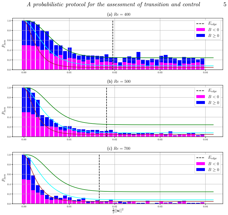
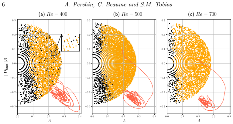
The carrying object is the laminarization-probability curve $P_{\mathrm{lam}}(E)$, estimated by Monte Carlo sampling over a random perturbation ensemble at each of 40 energy levels up to $(2/3)E_{\mathrm{turb}}$. Each random perturbation is built as $u = A u_\perp + B U_{\mathrm{lam}}$, with $u_\perp$ an incompressible field orthogonal to the laminar flow, spectral coefficients drawn uniformly, $B$ drawn uniformly from $[-2E/\|U_{\mathrm{lam}}\|, 2E/\|U_{\mathrm{lam}}\|]$, equal numbers of positive and negative $B$, and $A$ fixed by the energy constraint. The perturbations are integrated forward until their energy drops below $E_{\mathrm{lam}} = E_{\mathrm{turb}}/100$ (laminarization) or exceeds $E_{\mathrm{turb}}$ (transition); the empirical fraction at each energy is the probability. The fit $p(E) = 1 - (1-a)\gamma(\alpha,\beta E)$ with the lower incomplete gamma function compresses each curve into three parameters, making controlled and uncontrolled cases quantitatively comparable.
What would settle it
Recompute the laminarization-probability curves using a different, physically motivated perturbation family—for example, perturbations localised in the wall-normal direction or optimised for transient energy growth—and check whether the controlled curve still lies above the uncontrolled one at Re = 500; if the ordering reverses, the protocol's verdict is not robust.
Extended reading notes
Core claim
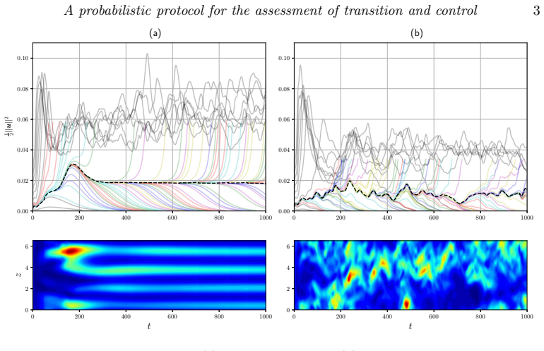
The central claim is that the robustness of the laminar state, and therefore the success of a control strategy, should be quantified by the probability that random finite-amplitude perturbations of a given energy return to laminar flow. In uncontrolled plane Couette flow, the laminarization probability $P_{\mathrm{lam}}(E)$ decreases from about 1 at small perturbation energies and saturates at a plateau $a$, with fitted values $a = 0.244$, $0.0805$, and $0.0484$ at Re = 400, 500, and 700. With spanwise wall oscillations of amplitude $W = 0.3$ and frequency $\omega = 1/16$ at Re = 500, the plateau rises to $0.286$ and the average relative increase of $P_{\mathrm{lam}}$ across the sampled energy range is 1.8, while the edge-state energy falls from roughly $1.82\times10^{-2}$ to $1.15\times10^{-2}$. Because the scalar indicators move in the opposite direction from the basin expansion, the paper argues that they cannot reliably assess control and that the full probability curve is required.
Load-bearing premise
The conclusion that wall oscillations suppress transition rests on the assumption that the randomly generated perturbation family used in the sampling is representative of the perturbations that would actually trigger transition in a real flow; the authors note this is a modelling choice.
Editorial extensions
If this is right
- Control assessment in subcritical shear flows should be based on energy-resolved laminarization probabilities rather than on edge-state or minimal-seed energies alone.
- At Re = 500, spanwise wall oscillations with amplitude 0.3 and frequency 1/16 nearly double the average laminarization probability, with the largest gains for large-energy perturbations.
- The controlled flow at Re = 500 behaves like the uncontrolled flow at Re = 400, except that small-energy perturbations are unaffected by the control.
- The fitting form $p(E) = 1 - (1-a)\gamma(\alpha,\beta E)$ provides a compact way to compare the effect of a control strategy at a given Reynolds number.
- The same sampling protocol can be applied to any system with finite-amplitude instability, including other shear flows and non-fluid multistable systems.
Reading between the lines
- If the protocol is right, a control study that reports only edge-state energy could reject a strategy that actually expands the laminar basin, since the edge-state energy here falls by about 37% while the laminarization probability rises.
- The sensitivity of the curves to the perturbation family suggests a robustness test: repeat the sampling with perturbations shaped like experimental noise or optimal transient-growth disturbances, and treat agreement between families as evidence for the control verdict.
- The non-zero plateau at large energies reflects the fractal interleaving of laminar and turbulent basins, so the protocol measures basin geometry as well as basin volume; a natural extension is to compute an energy-resolved basin-stability map for other multistable systems.
Signed reviews
Editorial analysis
A structured set of objections, weighed in public.
Referee Report
Summary. The paper proposes a probabilistic protocol for assessing the robustness of the laminar state and the efficacy of transition-control strategies. For plane Couette flow, the authors sample random initial perturbations at discrete kinetic-energy levels and estimate the laminarization probability Plam(E) as the fraction of trajectories that decay below an energy threshold. The uncontrolled results at Re = 400, 500, and 700 show a monotonically decreasing Plam(E) that saturates at a plateau value a, and the authors fit these curves with a reflected, saturated Gamma cumulative distribution function. They then apply the protocol to Re = 500 with spanwise wall oscillations (amplitude W = 0.3, frequency ω = 1/16), obtaining a plateau a = 0.286 versus a = 0.0805 uncontrolled, and report a mean relative increase in laminarization probability of 1.8. In contrast, the edge-state kinetic energy decreases by about 37% under control, which the authors interpret as demonstrating that scalar indicators such as edge-state or minimal-seed energy can be misleading for control assessment. The paper explicitly frames the work as a proof of concept and acknowledges that the perturbation family is a modeling choice.
Significance. If the result holds, the protocol offers a genuinely useful diagnostic for transition control: it replaces a single scalar criterion with an energy-resolved basin-stability measurement, and the controlled/uncontrolled comparison is made through direct numerical simulation rather than through the fitted curve. The paper is careful in its numerical methodology, uses standard edge-tracking and spectral DNS, and is explicit that the perturbation ensemble is a modeling choice. The main messages—that scalar proxies can disagree with the energy-resolved probability and that the protocol can be customized—are valuable and likely to influence subsequent work on transition control. The significance is tempered by the absence of statistical uncertainty quantification on the reported probabilities and by the fact that the headline control-effectiveness claim is demonstrated for one hand-chosen perturbation family only.
major comments (4)
- [Section 3, Fig. 4 and Table 1] The manuscript reports Plam values and fitted parameters without any uncertainty quantification. Plam(E) is a binomial proportion estimated from N = 100 or 200 independent draws, so the standard error at the uncontrolled plateau (a = 0.0805, N = 200) is about 0.019 and at the controlled plateau (a = 0.286, N = 200) about 0.032; the raw plateau difference is therefore large relative to sampling error, but the central quantitative claim of a 1.8-fold mean relative increase is computed from fitted Gamma CDFs and carries no confidence interval. Please add binomial confidence intervals (or at least the raw counts) for Plam at each energy level, report uncertainties for the fitted parameters a, α, and β, and state whether the 1.8 figure is statistically significant in the presence of multiple-comparison and fitting uncertainty.
- [Section 2 (RP generation) and Section 4 (Discussion)] The random perturbation family—uniform spectral coefficients, B drawn uniformly from [-2E/||Ulam||, 2E/||Ulam||] with equal numbers of positive and negative signs, and energies capped at (2/3)Eturb—is acknowledged in the Discussion to be a modeling choice, yet the abstract and Section 3 state that 'transition is significantly suppressed' without that qualifier. Because a different physically relevant perturbation family (for example, localized streamwise vortices or optimally growing disturbances) could in principle give a different ordering of the controlled and uncontrolled Plam curves, the central claim is strictly an ensemble-dependent result. Please either add a robustness test across perturbation families or systematically qualify the conclusion in the abstract and throughout as being valid for the chosen perturbation ensemble.
- [Section 2, Eq. (2.3), and Section 3 (controlled case)] In the controlled case the laminar base flow is time-dependent (spanwise wall oscillations), but the random perturbations are generated 'in the same way as for the uncontrolled case', i.e., using the steady profile Ulam = y ex, and the energy E is defined via Eq. (2.3) without specifying the reference state. The manuscript does not state whether u in the controlled case is the deviation from the oscillatory Stokes-layer solution or from Ulam. This distinction matters because the energy levels E(j), the thresholds Elam and Eturb, and the edge-state energy are all defined with respect to that decomposition. Please specify the reference base flow used in the controlled-case energy and perturbation generation, and if Ulam is retained, justify why that is the relevant state from which perturbations should be measured.
- [Section 3, relative probability increase] The 'relative probability increase' of 1.8 is defined as (posc(E) - p(E))/p(E) averaged over 'the range of the considered energies', but the averaging measure is not specified: uniform in E, uniform over the 40 discrete energy levels, or something else? The statistic is also computed from the fitted Gamma CDFs rather than directly from the measured Plam values. Please define the average precisely, report the corresponding raw-data statistic, and provide its sampling uncertainty.
minor comments (5)
- [Section 3, after 'laminarize'] The sentence beginning 'that of reducing the Reynolds number...' is a fragment and appears to be a vestige of an earlier draft; it should be completed or removed.
- [Section 4, first paragraph] There is a typo: 'Reynods' should be 'Reynolds'.
- [Section 3, controlled case] There is a typo: 'uncontroled' should be 'uncontrolled'.
- [Eq. (2.3)] The integral notation '∫_Ω u · u ∂Ω' appears to be a typo for 'dΩ' (or 'dV').
- [Section 3, fitting function] The notation γ(α, βE) for the lower incomplete gamma function is nonstandard; please define it explicitly as the regularized lower incomplete gamma function γ(α, βE)/Γ(α), so that p(E) is clearly a CDF.
Circularity Check
No significant circularity: the central controlled-vs-uncontrolled comparison is a direct numerical measurement, and the only self-citation is a non-load-bearing resolution reference.
full rationale
The paper's principal claim—that spanwise wall oscillation increases the laminarization probability and therefore suppresses transition—is established by direct numerical simulation: random perturbations are generated, integrated forward in time, and classified as laminarizing or transitioning according to energy thresholds. The laminarization probability Plam(E) is measured from these simulations, not derived from any fitted curve. The gamma cumulative distribution functions p(E) and posc(E) are descriptive least-squares fits to the measured probabilities, and the reported 1.8 relative increase is a summary of these fits; no quantity is presented as a prediction from first principles, so there is no fitted-input-called-prediction circularity. The only self-citation, to Pershin et al. (2019), is for the numerical resolution and domain size, which is not load-bearing for the control-efficiency conclusion. The authors also explicitly acknowledge in the Discussion that the choice of random perturbation form is a modeling decision and that the work is a proof of concept; this is a limitation on external validity, not a circular step. No equation is shown to be equivalent to an input by construction, and no load-bearing uniqueness theorem or ansatz is imported from the authors' prior work. The result is therefore self-contained against its own stated protocol, with at most a minor, non-circular self-citation.
Assumptions & free parameters
free parameters (5)
- a (plateau of laminarization probability) =
0.244, 0.0805, 0.0484, 0.286 (Re=400, 500, 700, controlled 500)
- alpha (gamma CDF shape) =
3.43, 2.05, 1.79, 3.75
- beta (gamma CDF rate) =
500, 412, 593, 899
- Classification thresholds Elam and tturb =
Elam = Eturb/100, tturb = 400 time units
- Energy window upper bound =
(2/3)Eturb = 0.04
assumptions (4)
- domain assumption Channelflow (Gibson 2014) with the stated spectral discretization accurately solves the incompressible Navier-Stokes equations for this flow.
- domain assumption The random perturbation ensemble (uniform spectral coefficients, uniform B, equal B signs) is representative of perturbations relevant to transition and control.
- domain assumption Turbulent lifetimes are at least an order of magnitude longer than tturb=400, so Plam is independent of the waiting time.
- domain assumption Edge tracking converges to the edge state, so Eedge values in Table 1 are reliable.
Cite this review
Pith. "Pith review of A probabilistic protocol for the assessment of transition and control." pith.science (2026). https://pith.science/paper/UR6Z46QE
@misc{pith2026190803050,
  author       = {Pith},
  title        = {Pith review of: A probabilistic protocol for the assessment of transition and control},
  year         = {2026},
  howpublished = {\url{https://pith.science/paper/UR6Z46QE}},
  note         = {Machine review of arXiv:1908.03050}
}
read the original abstract
Transition to turbulence dramatically alters the properties of fluid flows. In most canonical shear flows, the laminar flow is linearly stable and a finite-amplitude perturbation is necessary to trigger transition. Controlling transition to turbulence is achieved via the broadening or narrowing of the basin of attraction of the laminar flow. In this paper, a novel methodology to assess the robustness of the laminar flow and the efficiency of control strategies is introduced. It relies on the statistical sampling of the phase space neighborhood around the laminar flow in order to assess the transition probability of perturbations as a function of their energy. This approach is applied to a canonical flow (plane Couette flow) and provides invaluable insight: in the presence of the chosen control, transition is significantly suppressed whereas plausible scalar indicators of the nonlinear stability of the flow, such as the edge state energy, do not provide conclusive predictions. The methodology presented here in the context of transition to turbulence is applicable to any nonlinear system displaying finite-amplitude instability.
Figures
Figures from the paper (2 more)


Reference graph
Works this paper leans on
-
[1]
Avila, K. , Moxey, D. , de Lozar, A. , Avila, M. , Barkley, D. & Hof, B. 2011 The onset of turbulence in pipe flow . Science 333 (6039), 192--196
work page 2011
-
[2]
Baron, A. & Quadrio, M. 1995 Turbulent drag reduction by spanwise wall oscillations . Appl. Sci. Res. 55 (4), 311--326
work page 1995
-
[3]
Brunton, S. L. & Noack, B. R. 2015 Closed-loop turbulence control: progress and challenges . Appl. Mech. Rev. 67 (5)
work page 2015
-
[4]
Budanur, N. B. , Marensi, E. , Willis, A. P. & Hof, B. 2020 Upper edge of chaos and the energetics of transition in pipe flow . Phys. Rev. Fluids 5 (2), 023903
work page 2020
-
[5]
Canuto, C. , Hussaini, M. Y. , Quarteroni, A. & Zang, T. A. 1988 Spectral methods -- F undamentals in single domains . Springer-Verlag, New York
work page 1988
-
[6]
Chantry, M. & Schneider, T. M. 2014 Studying edge geometry in transiently turbulent shear flows . J. Fluid Mech. 747 , 506--517
work page 2014
-
[7]
Chantry, M. , Tuckerman, L. S. & Barkley, D. 2017 Universal continuous transition to turbulence in a planar shear flow . J. Fluid Mech. 824 , R1
work page 2017
-
[8]
Dauchot, O. & Daviaud, F. 1995 Finite amplitude perturbation and spots growth mechanism in plane C ouette flow . Phys. Fluids 7 (2), 335--343
work page 1995
Show all 46 references
-
[9]
, Brandt, L
Duguet, Y. , Brandt, L. & Larsson, B. R. J. 2010 Towards minimal perturbations in transitional plane C ouette flow . Phys. Rev. E 82 (2), 026316
2010
-
[10]
, Monokrousos, A
Duguet, Y. , Monokrousos, A. , Brandt, L. & Henningson, D. S. 2013 Minimal transition thresholds in plane C ouette flow . Phys. Fluids 25 (8), 084103
2013
-
[11]
, Lucarini, V
Faranda, D. , Lucarini, V. , Manneville, P. & Wouters, J. 2014 On using extreme values to detect global stability thresholds in multi-stable systems: The case of transitional plane C ouette flow . Chaos, Solitons & Fractals 64 , 26--35
2014
-
[12]
Gibson, J. F. 2014 Channelflow : A spectral Navier--Stokes simulator in C ++ . Tech. Rep.\/ . U. New Hampshire , Channelflow.org
2014
-
[13]
, De Lozar, A
Hof, B. , De Lozar, A. , Avila, M. , Tu, X. & Schneider, T. M. 2010 Eliminating turbulence in spatially intermittent flows . Science 327 (5972), 1491--1494
2010
-
[14]
, Westerweel, J
Hof, B. , Westerweel, J. , Schneider, T. M. & Eckhardt, B. 2006 Finite lifetime of turbulence in shear flows . Nature 443 (7107), 59
2006
-
[15]
, Mangiavacchi, N
Jung, W.-J. , Mangiavacchi, N. & Akhavan, R. 1992 Suppression of turbulence in wall-bounded flows by high-frequency spanwise oscillations . Phys. Fluids A-Fluid 4 (8), 1605--1607
1992
-
[16]
, Suzuki, Y
Kasagi, N. , Suzuki, Y. & Fukagata, K. 2009 Microelectromechanical systems--based feedback control of turbulence for skin friction reduction . Annu. Rev. Fluid Mech. 41
2009
-
[17]
2005 Laminarization of minimal plane C ouette flow: going beyond the basin of attraction of turbulence
Kawahara, G. 2005 Laminarization of minimal plane C ouette flow: going beyond the basin of attraction of turbulence . Phys. Fluids 17 (4), 041702
2005
-
[18]
, Kreilos, T
Khapko, T. , Kreilos, T. , Schlatter, P. , Duguet, Y. , Eckhardt, B. & Henningson, D. S. 2013 Localized edge states in the asymptotic suction boundary layer . J. Fluid Mech. 717 , R6
2013
-
[19]
, Kreilos, T
Khapko, T. , Kreilos, T. , Schlatter, P. , Duguet, Y. , Eckhardt, B. & Henningson, D. S. 2016 Edge states as mediators of bypass transition in boundary-layer flows . J. Fluid Mech. 801
2016
-
[20]
& Bewley, T
Kim, J. & Bewley, T. R. 2007 A linear systems approach to flow control . Annu. Rev. Fluid Mech. 39 , 383--417
2007
-
[21]
, Willis, A
Marensi, E. , Willis, A. P. & Kerswell, R. R. 2019 Stabilisation and drag reduction of pipe flows by flattening the base profile . J. Fluid Mech. 863 , 850--875
2019
-
[22]
, Meseguer, A
Mellibovsky, F. , Meseguer, A. , Schneider, T. M. & Eckhardt, B. 2009 Transition in localized pipe flow turbulence . Phys. Rev. Lett. 103 (5), 054502
2009
-
[23]
Menck, P. J. , Heitzig, J. , Marwan, N. & Kurths, J. 2013 How basin stability complements the linear-stability paradigm . Nat. Phys. 9 (2), 89--92
2013
-
[24]
, Faisst, H
Moehlis, J. , Faisst, H. & Eckhardt, B. 2004 A low-dimensional model for turbulent shear flows . New J. Phys. 6 (1), 56
2004
-
[25]
& Kerswell, R
Olvera, D. & Kerswell, R. R. 2017 Optimizing energy growth as a tool for finding exact coherent structures . Phys. Rev. Fluids 2 , 083902
2017
-
[26]
, Beaume, C
Pershin, A. , Beaume, C. & Tobias, S. M. 2019 Dynamics of spatially localized states in transitional plane C ouette flow . J. Fluid Mech. 867 , 414--437
2019
-
[27]
Pringle, C. C. T. , Willis, A. P. & Kerswell, R. R. 2012 Minimal seeds for shear flow turbulence: using nonlinear transient growth to touch the edge of chaos . J. Fluid Mech. 702 , 415--443
2012
-
[28]
Quadrio, Maurizio 2011 Drag reduction in turbulent boundary layers by in-plane wall motion . Philos. Trans. R. Soc. A 369 (1940), 1428--1442
1940
-
[29]
& Ricco, P
Quadrio, M. & Ricco, P. 2004 Critical assessment of turbulent drag reduction through spanwise wall oscillations . J. Fluid Mech. 521 , 251--271
2004
-
[30]
Rabin, S. M. E. , Caulfield, C. P. & Kerswell, R. R. 2014 Designing a more nonlinearly stable laminar flow via boundary manipulation . J. Fluid Mech. 738 , R1
2014
-
[31]
& Eckhardt, B
Schmiegel, A. & Eckhardt, B. 1997 Fractal stability border in plane C ouette flow . Phys. Rev. Lett. 79 (26), 5250
1997
-
[32]
Schneider, T. M. , Gibson, J. F. , Lagha, M. , De Lillo, F. & Eckhardt, B. 2008 Laminar-turbulent boundary in plane C ouette flow . Phys. Rev. E 78 (3), 037301
2008
-
[33]
, Avila, M
Shi, L. , Avila, M. & Hof, B. 2013 Scale invariance at the onset of turbulence in C ouette flow . Phys. Rev. Lett. 110 (20), 204502
2013
-
[34]
Skufca, J. D. , Yorke, J. A. & Eckhardt, B. 2006 Edge of chaos in a parallel shear flow . Phys. Rev. Lett. 96 (17), 174101
2006
-
[35]
Spalart, P. R. , Moser, R. D. & Rogers, M. M. 1991 Spectral methods for the Navier--Stokes equations with one infinite and two periodic directions . J. Comp. Phys. 96 (2), 297--324
1991
-
[36]
Sreenivasan, K. R. 1982 Laminarescent, relaminarizing and retransitional flows . Acta Mech. 44 , 1--48
1982
-
[37]
Stone, P. A. , Roy, A. , Larson, R. G. , Waleffe, F. & Graham, M. D. 2004 Polymer drag reduction in exact coherent structures of plane shear flow . Phys. Fluids 16 (9), 3470--3482
2004
-
[38]
Stone, P. A. , Waleffe, F. & Graham, M. D. 2002 Toward a structural understanding of turbulent drag reduction: nonlinear coherent states in viscoelastic shear flows . Phys. Rev. Lett. 89 (20), 208301
2002
-
[39]
, Gibson, J
Wang, J. , Gibson, J. & Waleffe, F. 2007 Lower branch coherent states in shear flows: transition and control . Phys. Rev. Lett. 98 (20), 204501
2007
-
[40]
, Iima, M
Watanabe, T. , Iima, M. & Nishiura, Y. 2016 A skeleton of collision dynamics: hierarchical network structure among even-symmetric steady pulses in binary fluid convection . SIAM J. Appl. Dyn. Sys. 15 (2), 789--806
2016
-
[41]
& Eckhardt, B
Zammert, S. & Eckhardt, B. 2015 Crisis bifurcations in plane P oiseuille flow . Phys. Rev. E 91 , 041003(R)
2015
-
[42]
, " * write output.state after.block = add.period write newline
ENTRY address author booktitle chapter edition editor howpublished institution journal key month note number organization pages publisher school series title type volume year eprint label extra.label sort.label short.list INTEGERS output.state before.all mid.sentence after.sen...
-
[43]
write newline
" write newline "" before.all 'output.state := FUNCTION n.dashify 't := "" t empty not t #1 #1 substring "-" = t #1 #2 substring "--" = not "--" * t #2 global.max substring 't := t #1 #1 substring "-" = "-" * t #2 global.max substring 't := while if t #1 #1 substring * t #2 gl...
-
[44]
@esa (Ref
\@ifclassloaded aguplus natbib The aguplus class already includes natbib coding, so you should not add it explicitly Type <Return> for now, but then later remove the command natbib from the document \@ifclassloaded nlinproc natbib The nlinproc class already includes natbib cod...
-
[45]
@stdbsttrue NAT@ctr \@lbibitem[ NAT@ctr ] \@lbibitem[#1]#2 \@extra@b@citeb \@ifundefined br@#2\@extra@b@citeb \@namedef br@#2 \@nameuse br@#2\@extra@b@citeb \@ifundefined b@#2\@extra@b@citeb @num @parse #2 [ @natanchorstart #2\@extra@b@citeb \@biblabel @num @natanchorend] @ifc...
-
[46]
@open @close @open @close and [1] URL: #1 \@ifundefined chapter * \@mkboth \@ifundefined NAT@sectionbib * \@mkboth * \@mkboth\@gobbletwo \@ifclassloaded amsart * \@ifclassloaded amsbook * \@ifundefined bib@heading @heading NAT@ctr thebibliography [1] @ \@biblabel NAT@ctr \@bib...
1996
Reviewed August 14, 2026 · model on record in the stance chip above.
Discussion (0). Continue with ORCID to comment.