REVIEW 3 major objections 5 minor 28 references
Explainable anomaly detection for sound spectrograms using pooling statistics with quantile differences
T0 review · 3 major / 5 minor · reviewed 2026-08-06 · deepseek-v4-flash
Pith's one-line read A per-pixel quantile rule detects machine sound anomalies as well as deep autoencoders on most machine types, with a built-in explanation map.
desk verdict A practical, explainable spectrogram anomaly detector that works reasonably on MIMII, but the 'theoretically founded' claim overreaches and needs a rewrite. read the letter →
The pith
A machine-rendered reading of the paper's core claim, the machinery that carries it, and where it could break.
The reading
What carries the argument
The load-bearing object is the reference spectrogram: a matrix of per-bin quantiles $q_j$ computed entry-wise over the normal training spectrograms, which serves as a boundary between 'normal' and 'suspicious' at every time-frequency location. The mechanism that carries the argument is the difference spectrogram $D=\max(0,W-Q)$, which isolates positive exceedances of a test spectrogram against that boundary and doubles as the explanation map. Four deviation metrics (Counting, Sum, Mean, Binomial) collapse $D$ into a single anomaly score, with the Binomial metric connected to theory: if each of $n$ independent bins exceeds its $z$-quantile with probability $1-z$, the number of exceedances follows $\mathrm{Bin}(n,1-z)$, so small binomial probabilities flag abnormal spectrograms. The authors also report an industrial-data check in which observed exceedance counts deviate from the binomial expectation by under one percent, while the variance is larger than the independent model predicts because neighboring frequencies and time windows are correlated.
What would settle it
Take a machine whose anormal samples are identical to normal ones except that one frequency band is attenuated by 10 dB, all else equal. Because $D=\max(0,W-Q)$ records only positive exceedances, the anomaly score for those samples would be nearly identical to normal samples and the ROC AUC would remain near 0.5; this would confirm that the one-sided quantile design, not the data difficulty, is the binding constraint.
Extended reading notes
Core claim
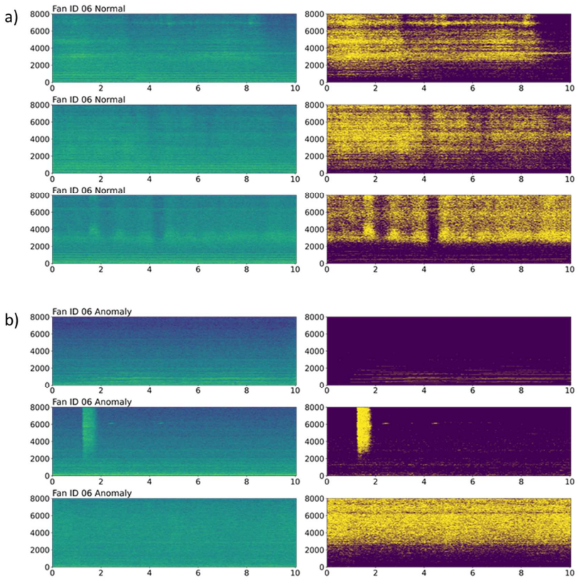
The central claim is that per-pixel quantile pooling is a sufficient basis for anomaly detection in sound spectrograms. For each bin $j$, the authors compute the $z$-quantile $q_j$ of that bin across the normal training spectrograms, forming a reference spectrogram $Q=(q_1,\dots,q_n)$. A test spectrogram $W$ is converted into a difference spectrogram $D=\max(0,W-Q)$, keeping only bins that exceed their reference value, and the anomaly score is one of four summaries of $D$: the number of nonzero bins, their sum, their mean, or a binomial probability that the observed count arose by chance. Under the idealized assumption of entry-wise independence, the count of exceedances is binomially distributed with $n$ trials and success probability $1-z$, which is the paper's theoretical justification for the score. On MIMII at 0 dB, the approach reaches AUC above 0.8 on 11 of 16 machine IDs and above 0.97 on four, and beats or matches the autoencoder baseline on 12 of 16 IDs; on the -6 dB recordings it is comparable to an image-transfer-learning method for pump, slider, and valve. The authors are explicit that the one-sided construction is the reason for the main failure case, fan ID 6, where anomalies appear not to raise the energy above normal levels.
Load-bearing premise
The load-bearing premise is that an anomalous sound manifests as a spectrogram bin with higher energy than the same bin's normal quantile; anomalies that are quieter, or that change patterns without raising amplitude, are invisible to this score.
Editorial extensions
If this is right
- A maintenance engineer gets a per-sample heatmap of exactly which time-frequency cells deviate from normal behavior, so the decision can be audited and root causes investigated.
- The method needs no gradient-based training, only a pass over normal samples to accumulate per-bin quantiles, so it can be deployed or re-calibrated quickly in a new plant.
- On the MIMII benchmark the method is on par or better than the autoencoder baseline on 12 of 16 machine IDs and on three of four machine types, suggesting that learned representations are not always necessary for this task.
- On the noisiest MIMII recordings (-6 dB) the method is comparable to an image-transfer-learning deep approach for pump, slider, and valve, despite being much simpler.
- Because the score must be tuned per machine and per noise level, the paper implies that a one-size-fits-all anomaly detector is not realistic for industrial sound monitoring.
Reading between the lines
- An immediate extension, which the paper names only as future work, is a two-sided version of the difference spectrogram using $|W-Q|$ or signed deviations; this would likely recover failure cases such as fan ID 6.
- Because neighboring time-frequency bins are correlated, the binomial anomaly probabilities are overconfident; computing an effective number of independent bins, or using permutation-based quantile tests, would sharpen the scores.
- The per-pixel quantile recipe transfers naturally to other grid-structured sensor data, such as vibration maps or thermal images, where an entry-wise 'normal envelope' is meaningful.
- The difference spectrogram could be compressed into recurring signatures (for example, periodic spikes at a fixed frequency) and used as features for a downstream classifier, turning the detector into an interpretable feature extractor.
Editorial analysis
A structured set of objections, weighed in public.
Referee Report
Summary. The manuscript proposes an explainable, non-learned anomaly detection method for machine sound spectrograms. From normal training spectrograms it computes an entry-wise z-quantile reference spectrogram; for a test spectrogram it forms the positive difference D = max(0, W - Q), then scores the result by counting, summing, averaging, or binomially weighting the positive entries. On the MIMII dataset at 0 dB, the authors report that the method matches or exceeds the autoencoder baseline in 12 of 16 machine settings and on average outperforms it on three of four machine types; on the -6 dB data they report competitive results with an image-transfer-learning approach. The paper also provides illustrative explainability outputs and an explicit discussion of the method's failure on fan ID 6.
Significance. The empirical core is genuinely useful for industrial anomaly detection: the method has only two hyperparameters, requires no learned representation, and yields per-pixel explanations, which is valuable in human-supervised settings. The evaluation protocol is reasonable, using separate training, validation, and test splits repeated over five seeds with hyperparameters tuned on validation only. The authors are candid about failure cases and noise effects. However, the paper's main theoretical justification is flawed as written: the binomial probability mass function is labeled as an anomaly probability, and the independence assumption behind it is acknowledged in Section 6 to be violated. If the authors rework Section 3.2 and the evidence in Section 6, the contribution as a simple, explainable, well-tested baseline remains worthwhile.
major comments (3)
- [Section 3.2] The displayed formula for P_anomaly(k,n) = C(n,k) * (1-z)^k * z^(n-k) is described as the probability that a test spectrogram does not belong to the training set distribution, but under the stated null hypothesis of a normal sample it is the probability of observing exactly k entries above their reference quantiles. Without a prior over anomaly mechanisms and a likelihood model for anomalous spectrograms, this quantity is not an anomaly probability. It can be used as a likelihood-based score or, with a tail sum, as a p-value under the null, and that would give a defensible theoretical motivation. In addition, because the reference entries Q_j are empirical quantiles from a finite training set, the equality P(W_j > Q_j) = 1 - z holds only asymptotically; the finite-sample nature of the quantile estimates should be acknowledged. This matters because 'theoretically founded' is a headline property in the abstract and conclusion.
- [Section 6] The experimental check of the binomial relation compares experimental mean deviation counts with the binomial expectation and reports roughly one percent relative bias. This validates the mean only, not the full distributional claim or the probability-of-anomaly interpretation. The final paragraph of Section 6 explicitly concedes that neighboring frequencies and time windows are highly correlated, so the i.i.d. assumption behind the binomial model is false. Please either validate the full distributional claim through measures such as variance, tail behavior, or a quantile-quantile analysis, or replace the exact binomial interpretation with an empirically calibrated scoring function and temper the theoretical language in Section 3.2 and Section 7 accordingly.
- [Sections 3.1 and 3.3; see also Section 5.3.2] The method is one-sided: D = max(0, W - Q), and Section 3.1 assumes an entry is anomalous only if it is higher than expected. Section 5.3.2 acknowledges that this assumption likely explains the poor fan ID 6 result (AUC 0.62 versus baseline 0.97), and the same limitation applies whenever an anomaly appears as unusually low energy or as a pattern change without higher amplitude. The paper should qualify its scope accordingly, for example by explicitly targeting 'positive-excitation anomalies' or by testing a two-sided variant, and the abstract and conclusion should not claim general anomaly detection without this caveat.
minor comments (5)
- [Section 4.4 and Table 2] The z-quantile grid is listed as {0.5, 0.6, 0.7, 0.8, 0.9, 0.95, 0.99}, but Table 2 reports 0.995 for fan ID 6 in splits 3 and 5; please clarify whether 0.995 was part of the search.
- [Section 5.1 and Figure 3] The averaged test AUCs are presented without variability; since each value is based on five random splits, please show error bars or confidence intervals and define what 'on par or better' means for the 12-out-of-16 claim.
- [Section 6] There is a typo in 'Incorpoarting', and the terms 'pixels' and 'deviation counts' should be explicitly mapped to the spectrogram entries defined in Section 3.2.
- [Section 7] The conclusion says the algorithm showed comparable or better detection performance compared with deep learning-based approaches, but the experiments compare only with the MIMII autoencoder baseline and the image-transfer-learning method of reference [15]; please restrict the claim to those specific comparisons.
- [Throughout] The paper consistently uses 'anormal', which is nonstandard in English; consider using 'anomalous' or defining the term at first use.
Circularity Check
No significant circularity: the quantile reference, difference spectrogram, and anomaly scores are defined directly from training data, hyperparameters are tuned on validation splits, and the binomial derivation follows from the quantile definition plus an explicit independence assumption rather than from the target result.
full rationale
The paper's derivation chain is self-contained and does not reduce to its own inputs. The reference spectrogram is computed as entry-wise z-quantiles over normal training spectrograms, and the difference spectrogram D = max(0, W - Q) is an explicit function of the test spectrogram and that reference. The Counting, Sum, Mean, and Binomial scores are defined directly from D or from the exceedance count k, not from fitted parameters that encode the test labels. Hyperparameters are selected on separate validation splits and final AUC is reported on held-out test splits, so no test-set fit is relabeled as prediction. The binomial PMF in Section 3.2 follows algebraically from the quantile definition and the stated entry-wise independence assumption; it is not a circular restatement of anomaly status, although the paper's interpretation of P_anomaly as 'the probability that a test spectrogram does not belong to the training set distribution' is statistically questionable. That concern, together with the one-sided anomaly assumption admitted in Section 5.3.2 and the violated i.i.d. assumption admitted in Section 6, is a validity or correctness issue rather than a circularity issue. The comparisons to the MIMII baseline and to the image-transfer-learning approach are external benchmarks, and the cited quantile-based works are not used as load-bearing justification for the central method. Overall, no step in the derivation is equivalent to its input by construction, so the appropriate finding is no significant circularity.
Assumptions & free parameters
free parameters (2)
- z-quantile =
0.9 to 0.99 (per machine/split)
- deviation metric =
Mean (mostly), Sum (one split)
assumptions (5)
- domain assumption Spectrogram entries are continuously distributed, so exactly a fraction 1-z of new normal samples exceed the z-quantile at each entry.
- domain assumption Entries of a spectrogram are independent across time and frequency.
- domain assumption Anomalies appear only as positive deviations above the normal quantile.
- domain assumption The training set contains only normal samples.
- domain assumption Published baseline AUCs are comparable across evaluation protocols.
Cite this review
Pith. "Pith review of Explainable anomaly detection for sound spectrograms using pooling statistics with quantile differences." pith.science (2026). https://pith.science/paper/USGQQSFK
@misc{pith2026250621921,
  author       = {Pith},
  title        = {Pith review of: Explainable anomaly detection for sound spectrograms using pooling statistics with quantile differences},
  year         = {2026},
  howpublished = {\url{https://pith.science/paper/USGQQSFK}},
  note         = {Machine review of arXiv:2506.21921}
}
read the original abstract
Anomaly detection is the task of identifying rarely occurring (i.e. anormal or anomalous) samples that differ from almost all other samples in a dataset. As the patterns of anormal samples are usually not known a priori, this task is highly challenging. Consequently, anomaly detection lies between semi- and unsupervised learning. The detection of anomalies in sound data, often called 'ASD' (Anomalous Sound Detection), is a sub-field that deals with the identification of new and yet unknown effects in acoustic recordings. It is of great importance for various applications in Industry 4.0. Here, vibrational or acoustic data are typically obtained from standard sensor signals used for predictive maintenance. Examples cover machine condition monitoring or quality assurance to track the state of components or products. However, the use of intelligent algorithms remains a controversial topic. Management generally aims for cost-reduction and automation, while quality and maintenance experts emphasize the need for human expertise and comprehensible solutions. In this work, we present an anomaly detection approach specifically designed for spectrograms. The approach is based on statistical evaluations and is theoretically motivated. In addition, it features intrinsic explainability, making it particularly suitable for applications in industrial settings. Thus, this algorithm is of relevance for applications in which black-box algorithms are unwanted or unsuitable.
Figures


Figures from the paper (8 more)




Reference graph
Works this paper leans on
-
[15]
Acoustic Anomaly Detection for Machine Sounds based on Image Transfer Learning,
R. Müller, F. Ritz, S. Illium, and C. Linnhoff-Popien, “Acoustic Anomaly Detection for Machine Sounds based on Image Transfer Learning,” Aug. 2022, pp. 49–56. Accessed: Aug. 22, 2022. [Online]. Available: https://www.scitepress.org/Link.aspx?doi=10.5220/0010185800490056
-
[1]
MIMII Dataset: Sound Dataset for Malfunctioning Industrial Machine Investigation and Inspection,
H. Purohit et al., “MIMII Dataset: Sound Dataset for Malfunctioning Industrial Machine Investigation and Inspection,” arXiv:1909.09347 [cs, eess, stat], Sep. 2019, Accessed: Dec. 21, 2021. [Online]. Available: http://arxiv.org/abs/1909.09347
arXiv 1909
-
[2]
An Introduction to Outlier Analysis,
C. C. Aggarwal, “An Introduction to Outlier Analysis,” in Outlier Analysis, C. C. Aggarwal, Ed. Cham: Springer International Publishing, 2017, pp. 1–34. doi: 10.1007/978-3-319-47578-3_1
-
[3]
V. Chandola, A. Banerjee, and V. Kumar, “Anomaly detection: A survey,” ACM Comput. Surv., vol. 41, no. 3, p. 15:1-15:58, Jul. 2009, doi: 10.1145/1541880.1541882
arXiv 2009
-
[4]
A review of novelty detection,
M. A. F. Pimentel, D. A. Clifton, L. Clifton, and L. Tarassenko, “A review of novelty detection,” Signal Processing, vol. 99, pp. 215–249, Jun. 2014, doi: 10.1016/j.sigpro.2013.12.026
-
[5]
Deep Learning for Anomaly Detection: A Survey,
R. Chalapathy and S. Chawla, “Deep Learning for Anomaly Detection: A Survey,” arXiv:1901.03407 [cs, stat], Jan. 2019, Accessed: Jan. 15, 2021. [Online]. Available: http://arxiv.org/abs/1901.03407
arXiv 1901
-
[6]
Deep Learning for Anomaly Detection: A Review,
G. Pang, C. Shen, L. Cao, and A. V. D. Hengel, “Deep Learning for Anomaly Detection: A Review,” ACM Comput. Surv., vol. 54, no. 2, p. 38:1-38:38, Mar. 2021, doi: 10.1145/3439950
doi:10.1145/3439950 2021
-
[7]
N. Ono et al., Proceedings of the 5th Workshop on Detection and Classication of Acoustic Scenes and Events (DCASE 2020). Zenodo, 2020. doi: 10.5281/zenodo.4061782
Show all 28 references
-
[8]
F. Font, A. Mesaros, D. P. W. Ellis, E. Fonseca, M. Fuentes, and B. Elizalde, Proceedings of the 6th Workshop on Detection and Classication of Acoustic Scenes and Events (DCASE 2021). Barcelona, Spain: Music Technology Group - Universitat Pompeu Fabra, 2021. doi: 10.5281/zenod...
2021 doi
-
[9]
Deep autoencoders for acoustic anomaly detection: experiments with working machine and in-vehicle audio,
G. Coelho, L. M. Matos, P. J. Pereira, A. Ferreira, A. Pilastri, and P. Cortez, “Deep autoencoders for acoustic anomaly detection: experiments with working machine and in-vehicle audio,” Neural Comput & Applic , May 2022, doi: 10.1007/s00521-022-07375-2
2022 doi
-
[10]
Deep Dense and Convolutional Autoencoders for Machine Acoustic Anomaly Detection,
G. Coelho et al., “Deep Dense and Convolutional Autoencoders for Machine Acoustic Anomaly Detection,” in Artificial Intelligence Applications and Innovations, Cham, 2021, pp. 337–348. doi: 10.1007/978-3-030-79150-6_27
2021 doi
-
[11]
ID-Conditioned Auto-Encoder for Unsupervised Anomaly Detection,
S. Kapka, “ID-Conditioned Auto-Encoder for Unsupervised Anomaly Detection,” arXiv:2007.05314 [cs, eess], Nov. 2020, doi: 10.5281/zenodo.4061782
2007 arXiv
-
[12]
Unsupervised Detection of Anomalous Sound based on Deep Learning and the Neyman-Pearson Lemma,
Y. Koizumi, S. Saito, H. U. Y. Kawachi, and N. Harada, “Unsupervised Detection of Anomalous Sound based on Deep Learning and the Neyman-Pearson Lemma,” IEEE/ACM Trans. Audio Speech Lang. Process., vol. 27, no. 1, pp. 212–224, Jan. 2019, doi: 10.1109/TASLP.2018.2877258
2019
-
[13]
Anomalous Sound Detection Using a Binary Classification Model and Class Centroids,
I. Kuroyanagi, T. Hayashi, K. Takeda, and T. Toda, “Anomalous Sound Detection Using a Binary Classification Model and Class Centroids,” in 2021 29th European Signal Processing Conference (EUSIPCO), Aug. 2021, pp. 1995–1999. doi: 10.23919/EUSIPCO54536.2021.9616198
2021
-
[14]
Anomalous Sound Detection as a Simple Binary Classification Problem with Careful Selection of Proxy Outlier Examples,
P. Primus, V. Haunschmid, P. Praher, and G. Widmer, “Anomalous Sound Detection as a Simple Binary Classification Problem with Careful Selection of Proxy Outlier Examples,” arXiv:2011.02949 [cs, eess], Nov. 2020, Accessed: Oct. 18, 2021. [Online]. Available: http://arxiv.org/ab...
2011 arXiv
-
[16]
Learning Deep Features for One-Class Classification,
P. Perera and V. M. Patel, “Learning Deep Features for One-Class Classification,” IEEE Transactions on Image Processing, vol. 28, no. 11, pp. 5450–5463, Nov. 2019, doi: 10.1109/TIP.2019.2917862
2019
-
[17]
Deep Residual Learning for Image Recognition,
K. He, X. Zhang, S. Ren, and J. Sun, “Deep Residual Learning for Image Recognition,” 2016, pp. 770–778. Accessed: Aug. 23, 2022. [Online]. Available: https://openaccess.thecvf.com/content_cvpr_2016/html/He_Deep_Residual_Learning_CVPR_2016_ paper.html
2016
-
[18]
Support Vector Method for Novelty Detection,
B. Schölkopf, R. C. Williamson, A. Smola, J. Shawe-Taylor, and J. Platt, “Support Vector Method for Novelty Detection,” in Advances in Neural Information Processing Systems, 1999, vol. 12. Accessed: Aug. 23, 2022. [Online]. Available: https://proceedings.neurips.cc/paper/1999/...
1999
-
[19]
Isolation Forest,
F. T. Liu, K. M. Ting, and Z.-H. Zhou, “Isolation Forest,” in 2008 Eighth IEEE International Conference on Data Mining, Dec. 2008, pp. 413–422. doi: 10.1109/ICDM.2008.17
2008 doi
-
[20]
Extreme value statistics for vibration spectra outlier detection,
A. Hazan, J. Lacaille, and K. K. Madani, “Extreme value statistics for vibration spectra outlier detection,” in International Conference on Condition Monitoring and Machinery Failure Prevention Technologies, Londres, United Kingdom, Jun. 2012, p. p.1. Accessed: Dec. 22, 2021. ...
2012
-
[21]
DCASE2020 Challenge - DCASE
“DCASE2020 Challenge - DCASE.” https://dcase.community/challenge2020/ (accessed Sep. 19, 2022)
2022
-
[22]
librosa: Audio and Music Signal Analysis in Python,
B. McFee et al., “librosa: Audio and Music Signal Analysis in Python,” Proceedings of the 14th Python in Science Conference, pp. 18–24, 2015, doi: 10.25080/Majora-7b98e3ed-003
2015 doi
-
[23]
Array programming with NumPy,
C. R. Harris et al., “Array programming with NumPy,” Nature, vol. 585, no. 7825, Art. no. 7825, Sep. 2020, doi: 10.1038/s41586-020-2649-2
2020 doi
-
[24]
The case against accuracy estimation for comparing induction algorithms
Provost, Foster J., et al. The case against accuracy estimation for comparing induction algorithms. in: ICML. 1998. S. 445-453
1998
-
[25]
SHEWHART CONTROL CHARTS
(2000). SHEWHART CONTROL CHARTS . In: Swamidass, P.M. (eds) Encyclopedia of Production and Manufacturing Management. Springer, Boston, MA. https://doi.org/10.1007/1-4020-0612- 8_874
2000 doi
-
[26]
Koenker, V
R. Koenker, V. Chernozhukov, X. He and L. Peng, (Eds.). (2017). Handbook of quantile regression
2017
-
[27]
Ditzhaus, R
M. Ditzhaus, R. Fried and M. Pauly, QANOVA: quantile-based permutation methods for general factorial designs. TEST, 2021, 30(4), 960-979
2021
-
[28]
Baumeister, M
M. Baumeister, M. Ditzhaus and M. Pauly, Quantile-based MANOVA: A new tool for inferring multivariate data in factorial designs. Journal of Multivariate Analysis, 2024, 199 , 105246
2024
Reviewed August 6, 2026 · model on record in the stance chip above.
Discussion (0). Continue with ORCID to comment.