REVIEW 3 major objections 6 minor 27 references
Clarifying species dependence under joint species distribution modeling
T0 review · 3 major / 6 minor · reviewed 2026-08-14 · deepseek-v4-flash
Pith's one-line read The paper argues that latent species correlations in joint species distribution models tell ecologists little about co-occurrence; the interpretable dependence lives in the induced odds ratios and their spatial surfaces.
desk verdict The core argument about latent correlations being uninformative for pairwise species dependence is correct and useful; the empirical odds-ratio surfaces are the soft spot but are illustrative rather than load-bearing. read the letter →
The pith
A machine-rendered reading of the paper's core claim, the machinery that carries it, and where it could break.
The reading
What carries the argument
The load-bearing object is the odds ratio for the $2 \times 2$ table of joint presence/absence, $\theta(s) = p_{00}(s)p_{11}(s)/(p_{10}(s)p_{01}(s))$ for a pair of species at location $s$, computed from probabilities induced by the latent model rather than modeled directly. In the spatial JSDM, presence is obtained by clipping a latent Gaussian process, $Y_j(s) = 1(Z_j(s) > 0)$, with $Z_j(s) = B x(s) + \Lambda W(s) + \epsilon(s)$, where a low-dimensional factor $W(s)$ follows independent Gaussian processes with a common exponential covariance; this is the dimension-reduced spatial specification that makes an $S$-by-$S$ covariance tractable and produces smooth probability surfaces. The appendix's monotonicity theorem, built on a classical bivariate-normal probability result, is what licenses the claim that latent correlation and odds ratio cannot have contradictory signs while also showing why the correlation magnitude is uninformative.
What would settle it
Numerical integration of the bivariate normal probabilities in (3) at fixed means and increasing $\rho$ would immediately falsify the theorem if it were not monotone; for the applied claim, a test is to fit the spatial JSDM and compare model-based odds-ratio surfaces against smoothed empirical odds ratios from the same sites: systematic sign reversals would indict the probit-threshold model, not the odds-ratio summary.
Extended reading notes
Core claim
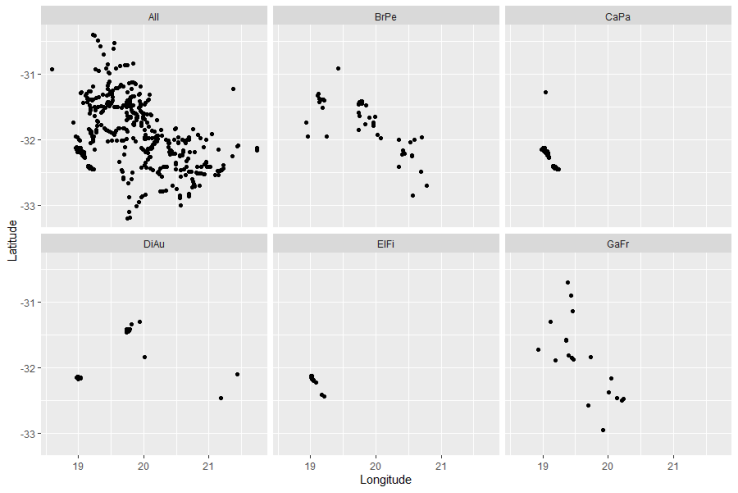
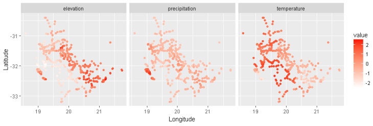
The paper's central claim is that dependence in a JSDM should be reported and interpreted through the $2 \times 2$ table of joint presence and absence for each species pair, not through the latent multivariate-normal correlation. For a pair of species at a site, let $\theta = p_{11}p_{00}/(p_{10}p_{01})$ be the odds ratio induced by thresholding the latent bivariate normal. The paper proves that with the latent means fixed, $\theta$ is non-decreasing in the latent correlation $\rho$, equals $1$ at $\rho = 0$, and the sign of $\log \theta$ matches the sign of $\rho$. Yet the magnitude of $\theta$ can be arbitrarily large or small for a fixed $\rho$ as the species means vary, and the joint occurrence probability can be large even with negative correlation. Consequently, the author argues, the $S \times S$ latent correlation matrix is a device for generating dependence but not an interpretable statement about it. The paper demonstrates the alternative by fitting a spatial JSDM to 639 tree species at 662 Cape Floristic Region sites and presenting posterior mean surfaces of $\log \theta$ for selected pairs, where positive-correlation pairs show regions of positive log odds ratios and negative-correlation pairs show regions of negative log odds ratios.
Load-bearing premise
The load-bearing premise is that the fitted probit-threshold latent-Gaussian model with a common spatial-decay parameter is a faithful generative description of the presence/absence data, so the odds-ratio surfaces it produces describe real ecological dependence rather than artifacts of the model.
Editorial extensions
If this is right
- Ecologists can replace the uninterpretable latent correlation matrix with maps of pairwise odds ratios, so that positive values mean co-occurrence or co-absence is encouraged and negative values mean it is discouraged.
- Because the odds ratio depends on the site-level mean probabilities, a single estimated correlation does not describe a species pair; the appropriate summary is a surface or a set of site-specific values.
- Spatial JSDM fitting smooths and interpolates these odds-ratio surfaces, so dependence at unsurveyed locations can be predicted.
- For ordinal abundance classifications, local, global, and cumulative odds ratios extend the same interpretation to abundance dependence; the paper notes that non-spatial JSDMs with counts could be handled this way.
- Stacked species distribution models, which assume independence, cannot represent sympatry or allopatry and will misstate the uncertainty in species richness even when expected richness agrees.
Reading between the lines
- Editorial inference: the monotonicity theorem transfers to any multivariate probit model, so disciplines that summarize binary-item dependence with tetrachoric correlations could adopt the same odds-ratio reporting.
- Editorial inference: a direct diagnostic for practitioners is to plot posterior odds-ratio surfaces against latent correlations; pairs with similar correlations but different prevalences should show visibly different dependence if the paper's caution is right.
- Editorial inference: a testable extension is to standardize the odds-ratio surface by each pair's marginal prevalence, separating rarity-driven absence from genuine avoidance.
Signed reviews
Editorial analysis
A structured set of objections, weighed in public.
Referee Report
Summary. The paper argues that in joint species distribution models (JSDMs) for presence/absence data, the latent multivariate normal correlation matrix is not a reliable guide to pairwise species dependence. Instead, the authors advocate reporting the induced odds ratios and joint occurrence probabilities, which have direct ecological interpretation. The central technical contribution is an appendix theorem, based on Slepian's theorem, showing that for fixed species means the odds ratio is non-decreasing in the latent correlation, equals 1 at zero correlation, and has the same sign as the correlation, yet its magnitude is strongly controlled by the mean occurrence probabilities. The paper proposes a spatial log-odds-ratio surface obtained from a spatial JSDM and illustrates it on Cape Floristic Region data for five selected species. It also discusses implications for species richness and sketches an extension to ordinal abundance data.
Significance. If the claims hold, the paper provides a useful corrective to the widespread practice of interpreting latent species correlations in JSDMs, and the proposed odds-ratio surface is a practical tool for ecologists. The appendix theorem is correct and cleanly supports the central interpretational message, and Figure 1 effectively demonstrates that latent correlation alone carries little information about dependence strength. The spatial odds-ratio surface is a constructive proposal that goes beyond merely criticizing the correlation view. However, the empirical demonstration is conditional on the adequacy of the fitted spatial JSDM, and one ancillary claim about maximum likelihood and expected richness is stated without proof. The paper is clearly written and the theorem is correctly derived.
major comments (3)
- [Section 3] The sentence "omitting details, maximum likelihood estimation will produce expectations that agree" is an unsupported assertion that is load-bearing for technical point (i) in the Introduction. Under the JSDM specification in Section 4, the marginal probability of presence is not generally equal to Phi(L^F); after integrating out the random effects it becomes E[Phi(L^F + L^R)], which depends on the random-effect variance. Unless the model is parameterized so that the marginal probabilities match those of the independent probit model, the expected richness under the joint and independent maximum likelihood fits need not agree. Please provide a proof or an explicit condition, qualify the claim, or remove it.
- [Section 5.1 and Section 6] The empirical odds-ratio surfaces are computed under a fitted model that assumes a common exponential spatial decay parameter for all latent factor processes. The paper asserts that the implications of this separable-model simplification "are expected to be negligible" (Section 5.1) but provides no supporting evidence or sensitivity analysis. Because the within-site species covariance is constant under this assumption, the reported log-odds-ratio surfaces in Figures 4 and 5 vary only through covariate-driven means; if true species-specific spatial ranges differ materially, the estimated factor loadings and implied pairwise correlations could be distorted. Please add a sensitivity check (e.g., fitting with r decay parameters, or comparing a subset of species under species-specific ranges) or explicitly temper the ecological conclusions drawn from the figures.
- [Section 6] The five species displayed in Figures 4 and 5 are selected post hoc to span a range of posterior correlations, and the surfaces are shown only as posterior means. Section 4.1 explains how to obtain posterior distributions for the odds ratios, yet no credible intervals or posterior probabilities of sign are reported. As a result, the qualitative claims in Section 6 (e.g., "large positive log theta(s) is observed in the western part") and the extreme value of -26.1 cannot be assessed for statistical precision or robustness to the species-selection rule. Please provide uncertainty summaries or at least explicitly note that these are illustrative posterior means without quantified uncertainty.
minor comments (6)
- [Section 4.1] Typo: "no direction connection" should be "no direct connection".
- [Section 1] The in-text citation "Wilkinson2018" should be formatted as "Wilkinson et al. (2018)".
- [Section 2] In the allopatry paragraph, the sentence "Switching the species, we have p11/p1. < p.1" appears to repeat the previous inequality; it should presumably read "p11/p.1 < p1.".
- [Figures 4 and 5] The captions use "parenthesis" where "parentheses" is meant.
- [Section 7] The display of the cumulative odds ratio definition is typeset ambiguously; the denominator should be a ratio of conditional probabilities for category k+1, not a product as it currently appears.
- [Section 2 and Figures 4/5] The paper states that log odds ratios are on the base-10 scale in Section 2, but Figures 4 and 5 do not specify the base; please state which logarithm is used in the figures so that the reported values (e.g., -26.1) are interpretable.
Circularity Check
No significant circularity: the odds-ratio surfaces are post-model-fitting transformations of fitted parameters, and the Appendix theorem is an independent mathematical result, not an input reused as an output.
full rationale
The paper's methodological claim is that latent correlations are difficult to interpret and that odds ratios and joint occurrence probabilities, induced by the fitted JSDM, are more interpretable. These odds ratios are defined in Eq. (3) as functions of the model parameters, and Section 4.1 explicitly treats them as post-model-fitting objects obtained from posterior samples. No parameter is fitted to the odds ratios themselves, so the reported surfaces are not a fitted input renamed as a prediction. The Appendix theorem, that the odds ratio is non-decreasing in the latent correlation for fixed means and that the sign of the log odds ratio matches the sign of the correlation, is proved from the standard Slepian and Gupta monotonicity results for bivariate normal probabilities; it is a genuine derivation rather than a restatement of the model definition. The spatial JSDM used for the Cape Floristic Region illustration is taken from Shirota et al. (2019), a self-citation, but the adequacy assumptions of that model, such as the common decay parameter discussed in Section 5.1, affect the reliability of the empirical illustration rather than reducing the central claim to the model's assumptions by construction. Concerns about the common-decay approximation being asserted as 'expected to be negligible' without supporting evidence are model-adequacy risks, not circularity under the stated criteria. Thus the derivation chain is self-contained for the paper's central technical claims.
Assumptions & free parameters
free parameters (5)
- Regression coefficient matrix B (S x p) =
not reported
- Factor loadings matrix Lambda (S x r) =
not reported
- Spatial GP decay parameter(s) =
not reported
- Number of latent factors r =
not stated (indicated as 3 to 5)
- Species selection threshold and five illustrated species =
at least 20 occurrences; correlations from -0.7 to 0.7
assumptions (6)
- standard math Slepian's theorem: bivariate normal rectangle probabilities are non-decreasing in correlation
- standard math Odds ratio properties: independence gives theta = 1; odds ratio is invariant to rescaling of the four cell probabilities
- domain assumption Presence/absence is generated by thresholding a latent multivariate normal (functional probit specification)
- domain assumption Spatial dependence of latent factors follows independent Gaussian processes with a common exponential covariance
- ad hoc to paper Maximum likelihood yields equal expected richness under independent and joint models
- domain assumption Realized presence/absence surfaces should be locally smooth
Cite this review
Pith. "Pith review of Clarifying species dependence under joint species distribution modeling." pith.science (2026). https://pith.science/paper/USPNCIKZ
@misc{pith2026190809410,
  author       = {Pith},
  title        = {Pith review of: Clarifying species dependence under joint species distribution modeling},
  year         = {2026},
  howpublished = {\url{https://pith.science/paper/USPNCIKZ}},
  note         = {Machine review of arXiv:1908.09410}
}
read the original abstract
Joint species distribution modeling is attracting increasing attention these days, acknowledging the fact that individual level modeling fails to take into account expected dependence/interaction between species. These models attempt to capture species dependence through an associated correlation matrix arising from a set of latent multivariate normal variables. However, these associations offer little insight into dependence behavior between species at sites. We focus on presence/absence data using joint species modeling which incorporates spatial dependence between sites. For pairs of species, we emphasize the induced odds ratios (along with the joint probabilities of occurrence); they provide much clearer understanding of joint presence/absence behavior. In fact, we propose a spatial odds ratio surface over the region of interest to capture how dependence varies over the region. We illustrate with a dataset from the Cape Floristic Region of South Africa consisting of more than 600 species at more than 600 sites. We present the spatial distribution of odds ratios for pairs of species that are positively correlated and pairs that are negatively correlated under the joint species distribution model. The multivariate normal covariance matrix associated with a collection of species is only a device for creating dependence among species but it lacks interpretation. By considering odds ratios, the quantitative ecologist will be able to better appreciate the practical dependence between species that is implicit in these joint species distribution modeling specifications.
Figures

Figures from the paper (2 more)


Reference graph
Works this paper leans on
-
[1]
Agresti, A. (2012). Categorical Data Analysis, 3rd Edition . Wiley
work page 2012
-
[2]
Anderson, R. P., D. Lewc, and A. T. Peterson (2002). Evaluating predictive models of species distributions: criteria for selecting optimal models. Ecological Modelling 162, 211–232
work page 2002
-
[3]
Banerjee, S., B. P. Carlin, and A. E. Gelfand (2014). Hierarchical Modeling and Analysis for Spatial Data, 2nd ed. Chapman and Hall/CRC
work page 2014
-
[4]
Brown, J. H., J. F. Gillooly, A. P. Allen, V. M. Savage, and G. B. West (2004). Toward a metabolic theory of ecology. Ecology 85, 1771–1789
work page 2004
-
[5]
Calabrese, J. M., G. Certain, C. Kraan, and C. F. Dormann (2014). Stacking species dis- tribution models and adjusting bias by linking them to macroecological models. Global Ecology and Biogeography 23, 99–112
work page 2014
-
[6]
Chib, S. (1998). Analysis of multivariate probit models. Biometrika 85 , 347–361
work page 1998
-
[7]
Clark, J. S., D. Nemergut, B. Seyednasrollah, P. Turner, and S. Zhange (2017). Generalized joint attribute modeling for biodiversity analysis: median-zero, multivariate, multifarious data. Ecological Monographs 87, 34–56
work page 2017
-
[8]
Cressie, N. and C. K. Wikle (2011). Statistics for Spatio-Temporal Data. Wiley. 20
work page 2011
Show all 27 references
-
[9]
Kaufman, J. T. Kerr, T. Oberdorff, E. O’Brien, and J. R. G. Turner (2004). Predic- tions and tests of climate-based hypotheses of broad-scale variation in taxonomic richness. Ecology Letters 7, 1121–1134. De Oliveira, V. (2000). Bayesian prediction of clipped gaussian random fie...
2004
-
[10]
Gelfand, A. E., A. M. Schmidt, S. Wu, J. A. Silander, A. Latimer, and A. G. Rebelo (2005). Modelling species diversity through species level hierarchical modelling. Journal of the Royal Statistical Society, Series C 54 , 1–20
2005
-
[11]
Gelfand, A. E. and S. Shirota (2019). Preferential sampling for presence/absence data and for fusion of presence/absence data with presence-only data. Ecological Monographs. DOI:10.1002/ecm.1372
2019 doi
-
[12]
Graham, C. H. and R. J. Hijmans (2006). A comparison of methods for mapping species ranges and species richness. Global Ecology and Biogeography 15, 578–587
2006
-
[13]
Guisan, A. and C. Rahbek (2011). SESAM - a new framework integrating macroecological and species distribution models for predicting spatio-temporal patterns of species assem- blages. Journal of Biogeography 38 , 1433–1444
2011
-
[14]
Gupta, S. S. (1963). Probability integrals of multivariate normal and multivariate t. Annals of Mathematical Statistics 34 , 792–828
1963
-
[15]
Latimer, A., S. Wu, A. E. Gelfand, and J. A. SilanderJr (2006). Building statistical models to analyze species distributions. Ecological Applications 16, 33–50
2006
-
[16]
Mueller-Dombois, D. and H. Ellenberg (1974). Aims and Methods of Vegetation Ecology . Wiley
1974
-
[17]
Abrego, P
Ovaskainen, O., N. Abrego, P. Halme, and D. Dunson (2016). Using latent variable models to identify large networks of species-to-species associations at different spatial scales.Methods in Ecology and Evolution 7 , 549–555
2016
-
[18]
Pineda, E. and J. M. Lobo (2009). Assessing the accuracy of species distribution models to predict amphibian species richness patterns. Journal of Animal Ecology 78 , 182–190
2009
-
[19]
Pollock, L. J., R. Tingley, W. K. Morris, N. Golding, R. B. O’Hara, K. M. Parris, P. A. Vesk, and M. A. McCarthy (2014). Understanding co-occurrence by modelling species 21 simultaneously with a Joint Species Distribution Model (JSDM). Methods in Ecology and Evolution 5 , 397–406
2014
-
[20]
Rebelo, T. (2001). SASOL Proteas: A Field Guide to the Proteas of South Africa (2nd ed). Fernwood Press
2001
-
[21]
Shirota, S., A. E. Gelfand, and S. Banerjee (2019). Spatial joint species distribution modeling using Dirichlet processes. Statistica Sinica 29 , 1127–1154
2019
-
[22]
Slepian, D. (1962). The one-sided barrier problem for Gaussian noise. Bell System Technical Journal 41 , 463–501
1962
-
[23]
Takhtajan, A. (1986). Floristic Regions of the World. University of California Press. Taylor-Rodr´ ıguez, D., K. Kaufeld, E. M. Schliep, J. S. Clark, and A. E. Gelfand (2017). Joint species distribution modeling: dimension reduction using Dirichlet processes. Bayesian Analysis...
1986
-
[24]
Thorson, J. T., M. D. Scheuerell, A. O. Shelton, K. E. See, H. J. Skaug, and K. Kristensen (2015). Spatial factor analysis: a new tool for estimating joint species distributions and correlations in species range. Methods in Ecology and Evolution 6 , 627–637
2015
-
[25]
Wilkinson, D. P., N. Golding, G. Guillera-Arroita, R. Tingley, and M. A. McCarthy (2018). A comparison of joint species distribution models for presenceabsence data. Methods in Ecology and Evolution 10 , 198–211
2018
-
[26]
Dormann, M. C. Forchhammer, J. Grytnes, A. Guisan, R. K. Heikkinen, T. T. Høye, I. K¨ uhn, M. Luoto, L. Maiorano, M. Nilsson, S. Normand, E. ¨ ockinger, N. M. Schmidt, M. Termansen, A. Timmermann, D. A. Wardle, P. Aastrup, and J. Svenning (2007). The role of biotic interaction...
2007
-
[27]
Zidek, J. V., W. Sun, and N. D. Le (1997). A decade of recovery of understory vegetation buried by volcanic tephra from mount st. helens. Ecological Monographs 67, 317–344. 22
1997
Reviewed August 14, 2026 · model on record in the stance chip above.
Discussion (0). Continue with ORCID to comment.