REVIEW 3 major objections 5 minor 70 references
Estimating Fe and Mg Abundances in the Milky Way Dwarf Galaxies Using Subaru/HSC and DEIMOS
T0 review · 3 major / 5 minor · reviewed 2026-08-06 · deepseek-v4-flash
Pith's one-line read Broad- and narrow-band photometry, calibrated by 610 spectra, yields reliable iron and magnesium abundances for 6,713 giants in four Milky Way dwarf galaxies and exposes radial abundance gradients that spectroscopy alone could not reach.
desk verdict Practical photometric abundance maps for four dSphs, but the headline outer-region gradients rest on extrapolated ML predictions and need radius-stratified validation. read the letter →
The pith
A machine-rendered reading of the paper's core claim, the machinery that carries it, and where it could break.
The reading
What carries the argument
The central object is a Random Forest regressor, an ensemble of decision trees whose predictions are averaged across trees, trained separately for [Fe/H] and [Mg/H]. Its input features are the absolute magnitudes $M_{g,0}$, $M_{i,0}$, $M_{NB515,0}$ and the colors $(g-i)_0$, $(g-NB515)_0$, and $(NB515-i)_0$, where the narrow $NB515$ band covers the Mg b triplet and is sensitive to surface gravity, allowing giant members to be separated from foreground dwarf stars and carrying much of the magnesium information. The model's per-star uncertainty comes from the tree-to-tree spread, and per-star prediction errors come from out-of-bag leaf-node root-mean-square errors; the most important features are $(NB515-i)_0$ for [Fe/H] and $(g-NB515)_0$ for [Mg/H].
What would settle it
Obtain medium-resolution spectra of a few dozen outer-region giant candidates in Fornax or Sculptor at predicted [Fe/H] near -2 and compare the measured abundances with the photometric predictions; a systematic offset comparable to the +0.74 dex overestimate already seen for the most metal-poor training stars would indicate that the outer gradients are calibration artifacts rather than real abundance patterns.
Extended reading notes
Core claim
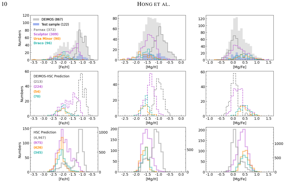
The central claim is that a Random Forest regressor trained on three HSC magnitudes and three color indices can predict spectroscopic-quality [Fe/H] and [Mg/H] for giants in Fornax, Sculptor, Ursa Minor, and Draco. Tested by five-fold cross-validation on 610 DEIMOS stars, the model achieves root-mean-square errors of 0.265 dex for [Fe/H] and 0.263 dex for [Mg/H], with mean out-of-bag errors of 0.289 and 0.306 dex. Applied to 6,713 HSC giants after rejecting twenty percent of candidates with large tree-to-tree model uncertainty, the predictions reproduce the central spectroscopic metallicity distribution functions and the [Mg/Fe] versus [Fe/H] patterns. The enlarged sample reveals negative radial abundance gradients in [Fe/H] and [Mg/H] extending out to roughly seven, nine, three, and four half-light radii for Fornax, Sculptor, Ursa Minor, and Draco respectively, with metal-poor and magnesium-rich stars increasingly common in the outskirts.
Load-bearing premise
The load-bearing premise is that a machine-learning model trained on 610 mostly central stars with measured spectra can be trusted to estimate iron and magnesium for all selected giants out to several half-light radii, including outer stars whose colors lie beyond the training distribution and whose ages may differ from the training stars.
Editorial extensions
If this is right
- Radial abundance gradients in these dwarf galaxies can now be measured to several half-light radii, revealing that metal-poor, magnesium-rich stars increasingly dominate the outskirts.
- The Fornax abundance distribution, with its extended metal-rich tail and a [Mg/Fe] bump near [Fe/H] = -1, supports a long, centrally concentrated star formation history with a gradual rise in Type Ia supernova enrichment.
- Sculptor's bimodal metallicity distribution and its central metal-rich concentration support a short, intense star formation episode in the periphery followed by more prolonged central enrichment.
- The shallow gradients of Ursa Minor and Draco are consistent with brief, intense star formation episodes that nearly extinguished star formation early, with Draco's slightly steeper gradient indicating a somewhat longer decline.
- The metal-poor end of the photometric distributions is systematically overestimated by about 0.74 dex for [Fe/H] below -2.5, so the most metal-poor photometric tail must be interpreted with caution.
Reading between the lines
- If the calibration transfers, the same pipeline could be applied to other dwarf galaxies already imaged by HSC, producing homogeneous abundance maps across the entire Milky Way satellite system without new spectroscopy.
- An untested but natural extension would be to break the age-metallicity degeneracy with isochrone-based stellar ages, which could separate first-generation populations from later enrichment episodes and directly test the bursty star formation interpretation.
- A direct observational test would be to take medium-resolution spectra of outer-region giants in Fornax or Sculptor, where the predicted [Fe/H] values fall near -2, and compare the measured abundances with the photometric predictions; a systematic offset similar to the metal-poor training bias would indicate the outer gradients are calibration artifacts.
- Adding a metallicity-sensitive filter such as NB395, which covers the Ca II H and K lines, would likely reduce the metal-poor overestimation and sharpen the inferred low-metallicity tails, a testable upgrade to the current method.
Editorial analysis
A structured set of objections, weighed in public.
Referee Report
Summary. The paper trains a Random Forest regressor on 610 DEIMOS spectroscopic measurements of [Fe/H] and [Mg/H] matched to Subaru/HSC photometry (g, i, NB515) for four Milky Way dwarf spheroidal galaxies (Fornax, Sculptor, Ursa Minor, Draco), and applies it to 6,713 HSC-selected giant candidates. It reports radial gradients in [Fe/H], [Mg/H], and [Mg/Fe] extending to roughly 7 half-light radii in Fornax, and uses these gradients plus abundance distribution shapes to infer differing star formation histories: extended formation in Fornax, shorter enrichment in Sculptor, and brief intense bursts in Ursa Minor and Draco. The paper also compares the photometric abundance distributions and [Mg/Fe] trends with prior spectroscopic results for the central regions.
Significance. If the photometric abundance estimates are reliable, the paper would deliver a substantial enlargement of the sample of chemically characterized stars in classical dSphs, reaching radii previously inaccessible to spectroscopy. The use of the NB515 narrow-band filter to constrain Mg and surface gravity is well motivated, and the authors are honest about known biases, including metal-poor overestimation and regression toward the mean. Machine-checked aspects are limited, but the paper does provide quantitative test metrics, out-of-bag error estimates, and a model-uncertainty exclusion criterion. However, the headline scientific claim—the outer-region radial gradients—rests on applying a model trained on predominantly central spectroscopic stars to stars far beyond the training footprint, and this is not yet validated by radius-stratified tests. The central-region agreement with earlier spectroscopy is a genuine strength, but it does not by itself establish the extrapolated gradients.
major comments (3)
- [§2.2, §4, Figs. 10–12] The central claim of new radial gradients beyond the spectroscopic footprint is not adequately validated. The Random Forest is trained on 610 DEIMOS stars that are strongly concentrated in the central regions (Fig. 10), and the paper itself concedes in §4 that the outermost [Fe/H] values near −2 'lie beyond the coverage of the DEIMOS sample and may therefore result from extrapolation.' Since §3.1 reports a mean residual of +0.74 dex for the 15 OOB stars with [Fe/H] ≤ −2.5, a radial trend in this bias could produce the apparent gradients even if the underlying metallicity distribution were flat. The authors should add a radius-stratified validation: for example, train on central stars only and test on the relatively outer DEIMOS stars, or bin the OOB/test residuals by galactocentric radius and show that the bias does not grow outward. They should also show how the metal-poor bias, if applied to the outskirts, would change the slopes in Figs. 11–12.
- [Table 1, §3.1, Fig. 8] The predictive power for [Mg/H] is weak: the test-set R² is 0.497 and the RMSE is 0.263 dex. Since [Mg/Fe] is computed by subtracting two predicted quantities, its accuracy is not independently validated, and §3.1 documents a −0.315 dex bias for stars with [Mg/H] > −0.8. Given that parts of the discussion (e.g., the α-knee and SFH interpretations in §4) rely on [Mg/Fe] trends, the authors should either quantify how the measured biases propagate into the claimed [Mg/Fe] gradients or soften the conclusions until a validation of [Mg/Fe] gradient recovery is provided.
- [Figs. 11 and 12] The radial gradient slopes are presented without uncertainties. Statements such as 'the slope ... does not differ significantly from the slope measured from the center outward' (Fornax) and comparisons between galaxies (e.g., 'Dra ... falls between those of UMi and Scl') are not supported without error bars on the slopes. The authors should report slope uncertainties, ideally from bootstrap resampling that accounts for the finite size and correlated nature of the photometric samples, and use these to test whether the inner and outer slopes are actually consistent.
minor comments (5)
- [§2.2] The description of the model uncertainty cut ('samples with model uncertainty greater than the maximum model uncertainty observed in the training sample were excluded') means that the threshold is defined by the training set; this should be stated more explicitly because it affects the comparison of training and test estimates.
- [§5] The text 'more ten times larger than our spectroscopic dataset' should read 'more than ten times larger'; the typo appears in the summary.
- [§4, Fig. 9] The statement that predictions 'beyond the dashed lines ... continue to follow similar trends' is made without a quantitative comparison. A simple metric, such as median [Mg/Fe] or [Fe/H] inside versus outside the DEIMOS footprint in matched bins, would strengthen the claim.
- [§3.4, Table 2] Because the model compresses the abundance range, the mean and standard deviation of the HSC predictions in Table 2 cannot be interpreted as unbiased estimates of the underlying stellar population; the authors should explicitly caution that the quoted widths are affected by regression toward the mean, particularly for [Mg/H].
- [§1] The filter name is typeset variously as 'N B515', 'NB515', and 'N B515'; using a consistent notation (e.g., NB515) throughout would improve readability.
Circularity Check
No significant circularity: the photometric abundance estimates and radial gradients are supervised outputs of an RF trained on DEIMOS abundances, but the gradients are not fitted targets and the paper's acknowledged outer-region extrapolation is a validity concern, not a definitional circularity.
full rationale
The derivation chain is an empirical calibration, not a self-referential loop. The RF regressors map HSC photometry (three magnitudes and three colors) to [Fe/H] and [Mg/H] using 610 DEIMOS spectroscopic labels; the 6713 HSC predictions are evaluated on photometry that was not used to set the abundance targets, and the radial gradients (Figs. 11-12) are least-squares slopes computed from those predicted abundances rather than quantities fitted to produce the gradients. No equation in the paper defines the predicted abundance in terms of the gradient, and no fitted parameter is renamed as a prediction. The paper explicitly flags the main threat in Section 4: photometric [Fe/H] near -2 in the outer regions 'lie beyond the coverage of the DEIMOS sample and may therefore result from extrapolation,' and Section 3.1 documents a +0.74 dex mean residual for the 15 out-of-bag stars with [Fe/H] <= -2.5. These are external-validity and extrapolation risks for the novel gradient claim, not circularity: the model output is not equivalent to its input by construction. Self-citations (Kirby et al. 2010, 2011a,b; Henderson et al. 2025; Komiyama et al. 2018b; Ogami et al. 2025) supply training spectra, selection methods, and comparison data, but none is invoked as a uniqueness theorem or as the sole justification for a conclusion; the central-region agreement is checked against independent spectroscopic studies. Accordingly, no circular step meets the evidentiary bar of exhibiting a specific reduction of a result to its inputs.
Assumptions & free parameters
free parameters (4)
- Random Forest hyperparameters (n_estimators, min_samples_leaf) =
500, 1
- Model uncertainty exclusion threshold =
maximum in-sample OOB model uncertainty, retaining 80% of HSC sample
- Proper motion sigma-clipping widths =
sigma = 3 (Fnx), 2 (Scl), 1.5 (UMi, Dra)
- Color-color polygon boundaries =
dashed polygons in Figure 1, different for Fornax
assumptions (5)
- domain assumption The NB515 narrow-band filter measures the Mg b triplet and is sensitive to surface gravity, so color-color cuts separate red giant members from foreground dwarfs.
- domain assumption The spectroscopic DEIMOS abundances used as training labels are accurate and unbiased across the full metallicity range.
- ad hoc to paper The photometric abundance relation learned by the Random Forest in the central, spectroscopically sampled regions holds in the outer regions beyond the DEIMOS footprint.
- domain assumption The age-metallicity degeneracy does not seriously bias photometric abundance predictions; combining all four galaxies without age information performed as well as age-dependent alternatives.
- domain assumption Stars in each galaxy share the same distance modulus from McConnachie (2012), and Gaia proper motion filtering removes foreground contamination.
Cite this review
Pith. "Pith review of Estimating Fe and Mg Abundances in the Milky Way Dwarf Galaxies Using Subaru/HSC and DEIMOS." pith.science (2026). https://pith.science/paper/UTBJRRZ4
@misc{pith2026250615952,
  author       = {Pith},
  title        = {Pith review of: Estimating Fe and Mg Abundances in the Milky Way Dwarf Galaxies Using Subaru/HSC and DEIMOS},
  year         = {2026},
  howpublished = {\url{https://pith.science/paper/UTBJRRZ4}},
  note         = {Machine review of arXiv:2506.15952}
}
read the original abstract
We investigate the chemical abundance distributions of the Fornax, Sculptor, Ursa Minor, and Draco dwarf galaxies using Subaru/HSC photometric data. The HSC dataset, which includes broadband g and i filters and the narrowband NB515 filter, offers sensitivity to iron and magnesium abundances as well as surface gravity, enabling the identification of giant stars and foreground dwarfs. For analysis, we selected a total of 6713 giant candidates using a Random Forest regressor trained on medium-resolution (R ~ 6000) Keck/DEIMOS spectroscopic data. Our analysis reveals the extent of radial metallicity gradients in the galaxies. Such trends, not detectable in earlier studies, are now captured owing to the substantially enlarged sample size and areal coverage provided by the HSC data. These results are also consistent with chemical abundance patterns previously observed in the central regions through spectroscopic studies. Furthermore, we infer that Fornax underwent extended star formation, whereas Sculptor formed both metal-poor and metal-rich stars over a shorter time. Ursa Minor and Draco appear to have experienced brief, intense star formation episodes leading to nearly extinguished star formation. This study underscores the critical role of the expanded HSC dataset in revealing chemical gradients that were previously inaccessible. Future work incorporating additional spectra of metal-poor stars and age-sensitive isochrone modeling will enable more accurate maps of chemical abundance distributions.
Figures


Figures from the paper (9 more)




Reference graph
Works this paper leans on
-
[1]
O., Chiti, A., Limberg, G., et al
Barbosa, F. O., Chiti, A., Limberg, G., et al. 2025, arXiv e-prints, arXiv:2504.03593, doi: 10.48550/arXiv.2504.03593
-
[2]
2006, A&A, 459, 423, doi: 10.1051/0004-6361:20065720
Battaglia, G., Tolstoy, E., Helmi, A., et al. 2006, A&A, 459, 423, doi: 10.1051/0004-6361:20065720
-
[3]
2014, arXiv e-prints, arXiv:1403.5237, doi: 10.48550/arXiv.1403.5237
Benitez, N., Dupke, R., Moles, M., et al. 2014, arXiv e-prints, arXiv:1403.5237, doi: 10.48550/arXiv.1403.5237
-
[4]
Bettinelli, M., Hidalgo, S. L., Cassisi, S., et al. 2019, MNRAS, 487, 5862, doi: 10.1093/mnras/stz1679
-
[5]
2015, arXiv e-prints, arXiv:1511.05741, doi: 10.48550/arXiv.1511.05741
Biau, G., & Scornet, E. 2015, arXiv e-prints, arXiv:1511.05741, doi: 10.48550/arXiv.1511.05741
-
[6]
2001, Machine Learning, 45, 5, doi: 10.1023/A:1010933404324
Breiman, L. 2001, Machine Learning, 45, 5, doi: 10.1023/A:1010933404324
-
[7]
Breiman, L., Friedman, J., Olshen, R., & Stone, C. J. 1984, Chapman and Hall/CRC
work page 1984
-
[8]
J., Moles, M., Crist´obal-Hornillos, D., et al
Cenarro, A. J., Moles, M., Crist´obal-Hornillos, D., et al. 2019, A&A, 622, A176, doi: 10.1051/0004-6361/201833036
Show all 70 references
-
[9]
G., & Huang, W
Cohen, J. G., & Huang, W. 2009, ApJ, 701, 1053, doi: 10.1088/0004-637X/701/2/1053 —. 2010, ApJ, 719, 931, doi: 10.1088/0004-637X/719/1/931
2009 doi
-
[10]
G., Da Costa, G
Coleman, M. G., Da Costa, G. S., & Bland-Hawthorn, J. 2005, AJ, 130, 1065, doi: 10.1086/432662 de Boer, T. J. L., Tolstoy, E., Hill, V ., et al. 2012a, A&A, 539, A103, doi: 10.1051/0004-6361/201118378 —. 2012b, A&A, 544, A73, doi: 10.1051/0004-6361/201219547 de los Reyes, M. A...
2005 doi
-
[11]
2013, The Messenger, 154, 32
Edge, A., Sutherland, W., Kuijken, K., et al. 2013, The Messenger, 154, 32
2013
-
[12]
P., & Sanders, J
Fallows, C. P., & Sanders, J. L. 2022, MNRAS, 516, 5521, doi: 10.1093/mnras/stac2550 Ferreira Lopes, C. E., Guti´errez-Soto, L. A., Ferreira Alberice, V . S., et al. 2025, A&A, 693, A306, doi: 10.1051/0004-6361/202451491
2022 doi
-
[13]
2018, PASJ, 70, S3, doi: 10.1093/pasj/psx079
Furusawa, H., Koike, M., Takata, T., et al. 2018, PASJ, 70, S3, doi: 10.1093/pasj/psx079
2018 doi
-
[14]
2020, ApJS, 247, 7, doi: 10.3847/1538-4365/ab6441
Han, S.-I., Kim, H.-S., Yoon, S.-J., et al. 2020, ApJS, 247, 7, doi: 10.3847/1538-4365/ab6441
2020 doi
-
[15]
R., Lian, J., et al
Hasselquist, S., Hayes, C. R., Lian, J., et al. 2021, ApJ, 923, 172, doi: 10.3847/1538-4357/ac25f9
2021 doi
-
[16]
J., Tibshirani, R
Hastie, T. J., Tibshirani, R. J., & Friedman, J. H. 2009, Springer 16 HONG ET AL
2009
-
[17]
E., Kirby, E
Henderson, L. E., Kirby, E. N., de los Reyes, M. A. C., Gerasimov, R., & Manwadkar, V . 2025, ApJ, 983, 117, doi: 10.3847/1538-4357/adbe7d
2025 doi
-
[18]
2014, A&A, 572, A82, doi: 10.1051/0004-6361/201424645
Hendricks, B., Koch, A., Walker, M., et al. 2014, A&A, 572, A82, doi: 10.1051/0004-6361/201424645
2014 doi
-
[19]
2019, A&A, 626, A15, doi: 10.1051/0004-6361/201833950
Hill, V ., Sk´ulad´ottir, ´A., Tolstoy, E., et al. 2019, A&A, 626, A15, doi: 10.1051/0004-6361/201833950
2019 doi
-
[20]
N., Chiba, M., et al
Hirai, Y ., Kirby, E. N., Chiba, M., et al. 2024, ApJ, 970, 105, doi: 10.3847/1538-4357/ad500c
2024 doi
-
[21]
C., Xiao, K., et al
Huang, Y ., Beers, T. C., Xiao, K., et al. 2024, ApJ, 974, 192, doi: 10.3847/1538-4357/ad6b94
2024 doi
-
[22]
2016, in Astronomical Society of the Pacific Conference Series, V ol
Jin, S., Irwin, M., Tolstoy, E., Lewis, J., & Hartke, J. 2016, in Astronomical Society of the Pacific Conference Series, V ol. 507, Multi-Object Spectroscopy in the Next Decade: Big Questions, Large Surveys, and Wide Fields, ed. I. Skillen, M. Balcells, & S. Trager, 241
2016
-
[23]
2018, PASJ, 70, 66, doi: 10.1093/pasj/psy056
Kawanomoto, S., Uraguchi, F., Komiyama, Y ., et al. 2018, PASJ, 70, 66, doi: 10.1093/pasj/psy056
2018 doi
-
[24]
N., Cohen, J
Kirby, E. N., Cohen, J. G., Guhathakurta, P., et al. 2013, ApJ, 779, 102, doi: 10.1088/0004-637X/779/2/102
2013 doi
-
[25]
N., Cohen, J
Kirby, E. N., Cohen, J. G., Smith, G. H., et al. 2011a, ApJ, 727, 79, doi: 10.1088/0004-637X/727/2/79
-
[26]
2011b, ApJ, 727, 78, doi: 10.1088/0004-637X/727/2/78
Guhathakurta, P. 2011b, ApJ, 727, 78, doi: 10.1088/0004-637X/727/2/78
-
[27]
N., Guhathakurta, P., Simon, J
Kirby, E. N., Guhathakurta, P., Simon, J. D., et al. 2010, ApJS, 191, 352, doi: 10.1088/0067-0049/191/2/352
2010 doi
-
[28]
2018a, PASJ, 70, S2, doi: 10.1093/pasj/psx069
Komiyama, Y ., Obuchi, Y ., Nakaya, H., et al. 2018a, PASJ, 70, S2, doi: 10.1093/pasj/psx069
-
[29]
2018b, ApJ, 853, 29, doi: 10.3847/1538-4357/aaa129
Komiyama, Y ., Chiba, M., Tanaka, M., et al. 2018b, ApJ, 853, 29, doi: 10.3847/1538-4357/aaa129
-
[30]
2019, A&A, 625, A2, doi: 10.1051/0004-6361/201834918
Kuijken, K., Heymans, C., Dvornik, A., et al. 2019, A&A, 625, A2, doi: 10.1051/0004-6361/201834918
2019 doi
-
[31]
Lemasle, B., de Boer, T. J. L., Hill, V ., et al. 2014, A&A, 572, A88, doi: 10.1051/0004-6361/201423919
2014 doi
-
[32]
2010, A&A, 523, A17, doi: 10.1051/0004-6361/200913413
Letarte, B., Hill, V ., Tolstoy, E., et al. 2010, A&A, 523, A17, doi: 10.1051/0004-6361/200913413
2010 doi
-
[33]
K., & Koch, A
Lianou, S., Grebel, E. K., & Koch, A. 2011, A&A, 531, A152, doi: 10.1051/0004-6361/201116998
2011 doi
-
[34]
2021, Journal of Machine Learning Research, 22, 1
Lu, B., & Hardin, J. 2021, Journal of Machine Learning Research, 22, 1
2021
-
[35]
2024, A&A, 686, A266, doi: 10.1051/0004-6361/202348093
Lucchesi, R., Jablonka, P., Sk´ulad´ottir, ´A., et al. 2024, A&A, 686, A266, doi: 10.1051/0004-6361/202348093
2024 doi
-
[36]
R., Ostheimer, J
Majewski, S. R., Ostheimer, J. C., Kunkel, W. E., & Patterson, R. J. 2000, AJ, 120, 2550, doi: 10.1086/316836
2000 doi
-
[37]
2010, ApJ, 722, 1879, doi: 10.1088/0004-637X/722/2/1879
Maoz, D., Sharon, K., & Gal-Yam, A. 2010, ApJ, 722, 1879, doi: 10.1088/0004-637X/722/2/1879
2010 doi
-
[38]
2006, MNRAS, 371, 643, doi: 10.1111/j.1365-2966.2006.10671.x Mart´ınez-Delgado, D., Alonso-Garc´ıa, J., Aparicio, A., & G´omez-Flechoso, M
Marcolini, A., D’Ercole, A., Brighenti, F., & Recchi, S. 2006, MNRAS, 371, 643, doi: 10.1111/j.1365-2966.2006.10671.x Mart´ınez-Delgado, D., Alonso-Garc´ıa, J., Aparicio, A., & G´omez-Flechoso, M. A. 2001, ApJL, 549, L63, doi: 10.1086/319150
2006
-
[39]
C., Crain, R
Mason, A. C., Crain, R. A., Schiavon, R. P., et al. 2024, MNRAS, 533, 184, doi: 10.1093/mnras/stae1743
2024 doi
-
[40]
McConnachie, A. W. 2012, AJ, 144, 4, doi: 10.1088/0004-6256/144/1/4
2012 doi
-
[41]
W., & Venn, K
McConnachie, A. W., & Venn, K. A. 2020, AJ, 160, 124, doi: 10.3847/1538-3881/aba4ab
2020 doi
-
[42]
1997, ARA&A, 35, 503, doi: 10.1146/annurev.astro.35.1.503 Mendes de Oliveira, C., Ribeiro, T., Schoenell, W., et al
McWilliam, A. 1997, ARA&A, 35, 503, doi: 10.1146/annurev.astro.35.1.503 Mendes de Oliveira, C., Ribeiro, T., Schoenell, W., et al. 2019, MNRAS, 489, 241, doi: 10.1093/mnras/stz1985
1997 doi
-
[43]
2012, in Society of Photo-Optical Instrumentation Engineers (SPIE) Conference
Miyazaki, S., Komiyama, Y ., Nakaya, H., et al. 2012, in Society of Photo-Optical Instrumentation Engineers (SPIE) Conference
2012
-
[44]
8446, Ground-based and Airborne Instrumentation for Astronomy IV , ed
Series, V ol. 8446, Ground-based and Airborne Instrumentation for Astronomy IV , ed. I. S. McLean, S. K. Ramsay, & H. Takami, 84460Z, doi: 10.1117/12.926844
-
[45]
2018, PASJ, 70, S1, doi: 10.1093/pasj/psx063
Miyazaki, S., Komiyama, Y ., Kawanomoto, S., et al. 2018, PASJ, 70, S1, doi: 10.1093/pasj/psx063
2018 doi
-
[46]
2020, ApJ, 905, 109, doi: 10.3847/1538-4357/abc486
Miyoshi, T., & Chiba, M. 2020, ApJ, 905, 109, doi: 10.3847/1538-4357/abc486
2020 doi
-
[47]
2024, ApJ, 971, 107, doi: 10.3847/1538-4357/ad5445
Ogami, I., Komiyama, Y ., Chiba, M., et al. 2024, ApJ, 971, 107, doi: 10.3847/1538-4357/ad5445
2024 doi
-
[48]
2025, MNRAS, 536, 530, doi: 10.1093/mnras/stae2527 ¨Ohman, Y
Ogami, I., Tanaka, M., Komiyama, Y ., et al. 2025, MNRAS, 536, 530, doi: 10.1093/mnras/stae2527 ¨Ohman, Y . 1934, ApJ, 80, 171, doi: 10.1086/143595
2025 doi
-
[49]
Okamoto, S., Ferguson, A. M. N., Arimoto, N., et al. 2024, ApJL, 967, L24, doi: 10.3847/2041-8213/ad4358 OpenAI,. 2024, ChatGPT-4o (May 13 version) [Large Language Model], https://chat.openai.com/chat
2024 doi
-
[50]
B., Erkal, D., & Li, T
Pace, A. B., Erkal, D., & Li, T. S. 2022, ApJ, 940, 136, doi: 10.3847/1538-4357/ac997b
2022 doi
-
[51]
B., Kaplinghat, M., Kirby, E., et al
Pace, A. B., Kaplinghat, M., Kirby, E., et al. 2020, MNRAS, 495, 3022, doi: 10.1093/mnras/staa1419
2020 doi
-
[52]
J., Hanke, M., et al
Reichert, M., Hansen, C. J., Hanke, M., et al. 2020, A&A, 641, A127, doi: 10.1051/0004-6361/201936930
2020 doi
-
[53]
F., Meisner, A
Schlafly, E. F., Meisner, A. M., & Green, G. M. 2019, ApJS, 240, 30, doi: 10.3847/1538-4365/aafbea Sch¨olkopf, B., Smola, A., & M¨uller, K.-R. 1998, Neural Computation, 10, 1299, doi: 10.1162/089976698300017467
2019 doi
-
[54]
A., et al
Sestito, F., Zaremba, D., Venn, K. A., et al. 2023, MNRAS, 525, 2875, doi: 10.1093/mnras/stad2427
2023 doi
-
[55]
D., Cˆot´e, P., & Sargent, W
Shetrone, M. D., Cˆot´e, P., & Sargent, W. L. W. 2001, ApJ, 548, 592, doi: 10.1086/319022
2001 doi
-
[56]
F., Cutri, R
Skrutskie, M. F., Cutri, R. M., Stiening, R., et al. 2006, AJ, 131, 1163, doi: 10.1086/498708 Sk´ulad´ottir, ´A., Vanni, I., Salvadori, S., & Lucchesi, R. 2024, A&A, 681, A44, doi: 10.1051/0004-6361/202346231 ESTIMATING PHOTOMETRICFE ANDMG OF DWARF GALAXIES17 Sk´ulad´ottir, ´A...
2006 doi
-
[57]
2010, A&A, 513, A34, doi: 10.1051/0004-6361/200913759
Starkenburg, E., Hill, V ., Tolstoy, E., et al. 2010, A&A, 513, A34, doi: 10.1051/0004-6361/200913759
2010 doi
-
[58]
2025, Research in Astronomy and Astrophysics, 25, 035001, doi: 10.1088/1674-4527/adb55b
Sun, B.-K., Chen, B.-Q., & Liu, X.-W. 2025, Research in Astronomy and Astrophysics, 25, 035001, doi: 10.1088/1674-4527/adb55b
2025 doi
-
[59]
S., Chiba, M., et al
Takada, M., Ellis, R. S., Chiba, M., et al. 2014, PASJ, 66, R1, doi: 10.1093/pasj/pst019
2014 doi
-
[60]
2023, A&A, 669, A125, doi: 10.1051/0004-6361/202244052
Tang, B., Zhang, J., Yan, Z., et al. 2023, A&A, 669, A125, doi: 10.1051/0004-6361/202244052
2023 doi
-
[61]
Thackeray, A. D. 1939, MNRAS, 99, 492, doi: 10.1093/mnras/99.6.492
1939 doi
-
[62]
2009, ARA&A, 47, 371, doi: 10.1146/annurev-astro-082708-101650
Tolstoy, E., Hill, V ., & Tosi, M. 2009, ARA&A, 47, 371, doi: 10.1146/annurev-astro-082708-101650
2009 doi
-
[63]
2023, A&A, 675, A49, doi: 10.1051/0004-6361/202245717
Tolstoy, E., Sk´ulad´ottir, ´A., Battaglia, G., et al. 2023, A&A, 675, A49, doi: 10.1051/0004-6361/202245717
2023 doi
-
[64]
2015, MNRAS, 449, 761, doi: 10.1093/mnras/stv294
Ural, U., Cescutti, G., Koch, A., et al. 2015, MNRAS, 449, 761, doi: 10.1093/mnras/stv294
2015 doi
-
[65]
Venn, K. A. 2014, Mem. Soc. Astron. Italiana, 85, 519
2014
-
[66]
G., Mateo, M., & Olszewski, E
Walker, M. G., Mateo, M., & Olszewski, E. W. 2009, AJ, 137, 3100, doi: 10.1088/0004-6256/137/2/3100
2009 doi
-
[67]
G., Mateo, M., Olszewski, E
Walker, M. G., Mateo, M., Olszewski, E. W., et al. 2007, ApJL, 667, L53, doi: 10.1086/521998
2007 doi
-
[68]
R., Dolphin, A
Weisz, D. R., Dolphin, A. E., Skillman, E. D., et al. 2014, ApJ, 789, 147, doi: 10.1088/0004-637X/789/2/147
2014 doi
-
[69]
L., Eisenhardt, P
Wright, E. L., Eisenhardt, P. R. M., Mainzer, A. K., et al. 2010, AJ, 140, 1868, doi: 10.1088/0004-6256/140/6/1868
2010 doi
-
[70]
2022, A&A, 659, A181, doi: 10.1051/0004-6361/202142724
Yang, L., Yuan, H., Xiang, M., et al. 2022, A&A, 659, A181, doi: 10.1051/0004-6361/202142724
2022 doi
Reviewed August 6, 2026 · model on record in the stance chip above.
Discussion (0). Continue with ORCID to comment.