Generalized Rellich's lemmas, uniqueness theorem and inside-out duality for scattering poles

Jiguang Sun; Lei Zhang; XiaoDong Liu

REVIEW 3 major objections 4 minor 22 references

Generalized Rellich's lemmas, uniqueness theorem and inside-out duality for scattering poles

T0 review · 3 major / 4 minor · reviewed 2026-08-06 · deepseek-v4-flash

Challenge this review Re-run · record.json Download PDF Read on arXiv ↗ Review JSON

Pith's one-line read Two generalized Rellich lemmas let a single far-field pattern at a complex wavenumber determine a sound-soft obstacle, and an inside-out duality turns scattering poles into blow-ups of an interior near-field equation.

desk verdict Worth reviewing: clean generalized Rellich lemmas and a real attempt at the pole-identification duality, but the numerics currently lag the theory on the indicator norm. read the letter →

arxiv 2507.04242 v1 pith:VF6HPV2Q submitted 2025-07-06 math.NA cs.NA

Xiaodong Liu , Jiguang Sun , Lei Zhang This is my paper · ORCID

classification math.NAcs.NA MSC 35P2535J0565N2135R30

keywords scatteringpolesresonancesRellich'slemmainverseuniquenessinside-outdualitylinearsamplingmethodHelmholtzequationcomplexwavenumber

verification ladder T0 review T1 audit T2 compute T3 formal

The pith

A machine-rendered reading of the paper's core claim, the machinery that carries it, and where it could break.

The reading

The paper proves two generalized Rellich lemmas that keep the classical principle 'decay at infinity forces a Helmholtz solution to vanish' alive for complex wavenumbers, provided the decay condition is weighted by an exponential factor. From these it derives a uniqueness theorem: a single far-field pattern measured at one non-real wavenumber identifies a sound-soft obstacle, a regime where the real-wavenumber problem is still open. The second half establishes an inside-out duality showing that the poles of the exterior Dirichlet or Neumann problem can be read off from an interior near-field equation: away from a pole the approximate solutions stay bounded in a natural energy norm, while at a pole that norm must blow up for almost every exterior sampling point. The paper verifies the criterion numerically on disks and ellipses, where the plotted density spikes match known poles closely, and notes that cornered domains are less accurate.

What carries the argument

The machinery that carries the argument is the spherical-harmonic expansion of an outgoing Helmholtz solution combined with the Hankel-function asymptotics (2.6); inserting the expansion into the weighted decay condition (2.9) shows that each coefficient must vanish, which is the content of the two generalized Rellich lemmas. For the pole characterization, the central object is the interior near-field operator $N_k:L^2(\partial\Omega)\to L^2(\partial\Omega)$ defined by (3.21), with the factorization $N_k=G_kS_k$, where $S_k$ is the single-layer potential on the measurement curve $\partial\Omega$ and $G_k$ maps the boundary data on $\partial D$ to the corresponding interior solution restricted to $\partial\Omega$. Theorems 3.3 through 3.6 turn the dense-range property of $S_k$ away from poles and a weak-compactness argument at a pole into the dichotomy: boundedness of $\|S_k g^{\varepsilon}_z\|_{H^1_{\mathrm{loc}}}$ for almost every $z$ characterizes non-poles, and its blow-up characterizes poles.

What would settle it

Take the unit disk, where the Dirichlet poles are known zeros of Hankel functions, and at one such pole measure the residual and the $H^1_{\mathrm{loc}}$ norm of $S_k g^{\varepsilon}_z$ for a decreasing sequence of regularization parameters; if the residual cannot be pushed to zero while the density norm grows, or if the energy norm stays bounded at a pole, the numerical pole-detection is operating outside the proven theorem.

Watch

Extended reading notes

Core claim

The paper's central claim is two-fold. On the far-field side, the outgoing scattered field and its far-field pattern are in one-to-one correspondence for every $k\in \mathbb{C}\setminus\mathbb{R}_{\le 0}$, not just positive real $k$. This is established through the generalized Rellich lemmas (Lemma 2.2 and Lemma 2.4), and it yields Theorem 2.6: two sound-soft obstacles with the same far-field pattern at a fixed non-real wavenumber, for a single plane wave or point source, must coincide; likewise, if they share a Dirichlet pole $k$ with a common nontrivial far-field pattern, they must coincide. On the pole side, the paper proves that the interior near-field operator $N_k=G_kS_k$ detects poles: for $k\in\mathbb{C}_-$ that is not a Dirichlet (or Neumann) pole, for any exterior point $z$ there are approximate solutions $g^{\varepsilon}_z$ to $N_k g=\Phi_k(\cdot,z)$ with $\|S_k g^{\varepsilon}_z\|_{H^1_{\mathrm{loc}}}$ bounded, whereas at a pole, under the convergence assumption (3.26) or (3.37), the norm cannot remain bounded for almost every $z$. This is the inside-out duality: the exterior pole forces an interior blow-up.

Load-bearing premise

The load-bearing assumption is that approximate solutions to the interior near-field equation can be found whose residual tends to zero for every exterior point $z$, and that the numerically plotted density norm faithfully represents the energy norm of $S_k g$ that the theory controls.

Editorial extensions

If this is right

A single far-field pattern at one non-real wavenumber uniquely determines the sound-soft obstacle, and the same conclusion holds at a common Dirichlet pole with nonzero far-field.
Dirichlet and Neumann scattering poles can be located by computing solutions of an interior near-field equation and watching the norm of the approximate density blow up.
When the wavenumber is not a pole, the interior near-field equation has approximate solutions with bounded energy norm, giving a stable non-pole regime that complements the blow-up criterion.
The generalized Rellich lemmas extend the far-field-pattern/scattered-field correspondence to all $k\in\mathbb{C}\setminus\mathbb{R}_{\le 0}$, so inverse obstacle scattering at complex wavenumbers sits on the same footing as the positive-real case.

Reading between the lines

Editorial extensions of the paper, not claims the author makes directly.

A natural test would replace the $\ell^2$ density norm with the $H^1_{\mathrm{loc}}$ norm of $S_k g$ that the theorems control; if the two indicators agree at poles, the numerical method becomes a proven pole detector.
The method requires the measurement curve $\partial\Omega$ to lie strictly inside the obstacle, so the practical setting is one with partial knowledge of the obstacle; fully exterior-only data would need a different formulation.
The corner-rounding experiment suggests interior data lose corner information; quantifying the pole shift as corners are rounded gives a testable signature of that loss.
Verifying the convergence assumption (3.26)/(3.37) for Tikhonov-regularized solutions is the natural next step; if it holds, the blow-up criterion is unconditional.

Share X Bluesky LinkedIn Reddit HN

Editorial analysis

A structured set of objections, weighed in public.

Desk editor's note, referee report, and a circularity audit.

Desk Editor's Note

read the letter

Dear colleague,

Quick take: this paper deserves a serious referee, but not as-is. The generalized Rellich lemmas (2.2, 2.4) and the far-field uniqueness theorem (2.5) are clean and correct. Theorem 2.6 is a genuine attempt to fix Labreuche's gap, though the proof has a technical hole the authors themselves flag: D* can have cusps, so Green's theorem is not guaranteed. That is fixable, but it should be stated as an assumption rather than left as a side remark.

The inside-out duality section is the most interesting and the least settled. Theorems 3.3-3.6 characterize poles by blow-up of ||S_k g|| in H^1_loc, but they are conditional on the convergence assumption (3.26)/(3.37). That is natural in the LSM framework, yet the paper never verifies it for the numerical scheme actually used. Also, the dense-range statement in Theorem 3.2 is overbroad: the range of S_k lies in the closed subspace of radiating solutions, so it cannot be dense in all of H^1_loc(R^2\D). The proof actually shows denseness in the radiating subspace, which is all the later arguments need—so this is a correctable error, not a fatal one.

The bigger gap is between theory and numerics. The theorems control ||S_k g|| in H^1_loc, but Section 4 plots the l2 norm of the Tikhonov density (Remark 4.1 openly substitutes). Because S_k is injective with non-closed range, an l2 spike is not logically tied to an H^1 blow-up. The numerical demonstrations are therefore heuristic. They are encouraging—spikes appear at known poles, and the corner-degradation discussion is honest—but they do not yet validate the theorem's precise claim. A referee should ask for either a numerical indicator with theoretical backing or a justification of why the l2 norm tracks the H^1 norm in practice.

That said, the paper is honest, well-written, and contributes real material: the generalized Rellich lemmas, the corrected uniqueness argument, and a clear presentation of the inside-out duality for both Dirichlet and Neumann cases. I would send it to review and ask for revisions on the points above. It deserves a serious referee.

Best, [Your name]

Referee Report

3 major / 4 minor

Summary. The paper studies acoustic scattering by sound-soft and sound-hard obstacles at complex wavenumbers with negative imaginary part. It proves two generalized Rellich lemmas for such wavenumbers, uses them to show that a vanishing far-field pattern forces the scattered field to vanish, and derives uniqueness theorems for inverse scattering from a single far-field pattern for non-real k, including a Dirichlet-pole case. It then develops an inside-out duality for scattering poles: when k is not a Dirichlet/Neumann pole, the interior near-field equation has approximate solutions with bounded H^1_loc norm of the single-layer potential S_k g, whereas when k is a pole and the near-field residuals converge, that H^1_loc norm must blow up for almost every exterior point z. Numerical experiments for disks, ellipses, and a square use a discretized Tikhonov-regularized near-field equation and plot the l2 norm of the density as a pole indicator. The paper concludes that exterior Dirichlet/Neumann poles can be identified from interior scattering data.

Significance. If fully established, the generalized Rellich lemmas and the uniqueness theorems would give new qualitative information about inverse scattering at complex frequencies, and the inside-out duality would provide a rigorous basis for computing scattering poles from interior near-field data, complementing the recent work of Cakoni, Colton, and Haddar and of Cakoni, Haddar, and Dana. The paper is clearly structured and contains explicit proofs of the factorization N_k = G_k S_k and of the dense-range/injectivity properties of the relevant operators. The authors are also honest about the reduced accuracy for domains with corners. The main weaknesses are the gap between the theorems, which control the H^1_loc norm of S_k g, and the numerical indicator, which is the l2 norm of the density, as well as several proof gaps in the uniqueness and pole-characterization arguments. The theoretical core is promising but the practical claim advertised in the abstract is not yet supported by the numerical evidence as presented.

major comments (3)

[Section 2.2, Theorem 2.6] The proof of Theorem 2.6 takes the imaginary part of Green's identity and claims that k in C\R implies the imaginary part yields u_2 = 0. This fails for purely imaginary k, since then k^2 is real and Im(k^2)=0; the imaginary part gives 0=0. For such k one should instead take the real part, since for k^2<0 the real part gives ∫(|∇u_2|^2 + |k|^2|u_2|^2)=0. Additionally, Green's theorem is applied to the domain D* although, as the authors themselves note a few lines later, D* may have cusps and Green's theorem may not hold there. The theorem may be true, but the proof needs to handle the purely imaginary case separately and to justify the integration by parts on D*, for instance by an approximation argument or by proving that the relevant boundary is admissible despite the cusps.
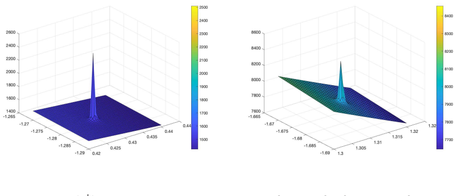
[Section 4 and Theorems 3.4/3.6, Remark 4.1] The theory characterizes poles by unboundedness of ||S_k g^eps_z||_{H^1_loc(R^2\D)} under the convergence assumptions (3.26)/(3.37), but the numerical implementation solves the discrete Tikhonov-regularized system (4.44) and plots the l2 norm |g_k| of the density, as Remark 4.1 openly states. These two quantities are not equivalent: S_k: L2(∂Ω) → H^1_loc is bounded and injective, but as a compact operator into H^1 on bounded subdomains it has non-closed range, so there exist sequences with ||g_n||_{L2} → ∞ while ||S_k g_n||_{H^1_loc} remains bounded. Thus an l2 spike can occur at a wavenumber where the theoretical quantity stays finite. The paper does not prove that the Tikhonov solutions satisfy the residual convergence (3.26)/(3.37), nor that the l2 norm tracks the H^1_loc norm. Since the abstract's practical claim that poles can be identified rests on the numerical spikes, the numerical demonstrations are currently outside the theory. The authors should either compute the H^1_loc norm of S_k g (or a justified proxy), verify that the residuals tend to zero, or substantially soften the claims.
[Theorems 3.4 and 3.6, proofs] In both proofs, after obtaining a weakly convergent sequence v_n := S_k g^{eps_n}_z, the authors introduce an outgoing solution ~v with prescribed Dirichlet boundary data v on ∂D (Theorem 3.4) or prescribed Neumann data Tv on ∂D (Theorem 3.6). At a scattering pole the exterior Dirichlet or Neumann problem is not well-posed, and it is not automatic that such an outgoing solution exists for every boundary datum v. The proofs need to justify that the weak limit v of the outgoing single-layer potentials is itself outgoing and can serve as ~v, or otherwise establish existence of the required outgoing solution. Without this, the contradiction argument is not complete.

minor comments (4)

[Section 2.2, Theorem 2.6 proof] The phrase 'the scattered field us grows (or decays) exponentially as |x| → 0' should read 'as |x| → ∞'.
[Section 3.2, proof of Theorem 3.6] The sentence 'Combination of (3.28) and (3.26)' should refer to (3.38) and (3.37), respectively; the preceding line also states that Tv_n converges in H^{1/2}(∂D) when the Neumann trace should be in H^{-1/2}(∂D).
[Section 4.2, Example 3] The first sound-hard disk pole is listed as 0.5012 − 6.4355i, but the search window is S = [0.49,0.51] × [−0.65,−0.63] and the reported spike is at 0.5018 − 0.6442i. The listed exact pole is not in the window, so the comparison is internally inconsistent; this appears to be a typo in the imaginary part of the exact pole and should be corrected.
[Abstract and Section 4] The claim that poles can be identified 'without prior knowledge of the actual sound-soft or sound-hard obstacles' is stronger than what is demonstrated: the method requires selecting a curve ∂Ω strictly inside the unknown obstacle D, so some interior information about D is assumed. The paper should qualify this in the abstract and introduction.

Circularity Check

0 steps flagged · score 2.0 of 10

No load-bearing circularity: the pole characterization is derived from factorization and dense-range arguments with no fitted parameters, and the same-group citations are validation benchmarks rather than derivation inputs; the main caveat is an acknowledged numerical heuristic (l2 norm instead of H1 norm).

full rationale

The derivation chain is self-contained. Lemmas 2.2 and 2.4 are coefficient-wise consequences of Hankel asymptotics, and Theorem 2.6 follows from Lemma 2.4 plus a Green-identity argument, not from the conclusion. Theorems 3.3 to 3.6 establish the inside-out duality from the factorization N_k = G_k S_k, the injectivity and dense-range properties of S_k in Theorem 3.2, and a contradiction using the pole eigenfunction; no parameter is fitted to the target poles, and conditions (3.26) and (3.37) are hypotheses, not re-statements of the conclusion. The cited Lemma 2.10 of [4] is external, from Cakoni, Colton, and Haddar, and the approximation result is also re-proved in Theorem 3.3 via Theorem 3.2. The only same-group citations are [15] and [22], used to supply ground-truth poles; for the disk these agree with independent Hankel-zero values, and the DtN computation is a different numerical method, so they do not feed back into the abstract characterization. Limitations are present but are not circularity: Remark 4.1 explicitly substitutes the l2 norm of g_k for the H1_loc norm of S_k g controlled by Theorems 3.4 and 3.6, Section 4.3 reports degraded accuracy for cornered domains, and Section 5 acknowledges that corner limitation; these are gaps between theory and numerics, not reductions of the theorems to their inputs. The abstract claim of identifying poles without prior knowledge is also tempered by the need to choose a closed curve inside the obstacle, but that is a methodological limitation rather than a circular step. The score is therefore low, with the small nonzero value reflecting only the minor non-load-bearing same-group validation dependence and the acknowledged heuristic indicator.

Assumptions & free parameters 2 free parameters · 9 assumptions · 0 invented entities

The central theorems introduce no fitted parameters and no invented entities. They rest on standard scattering facts (Green representation (2.4), Hankel asymptotics, analyticity of far fields, Holmgren's theorem, unique continuation), the standard observation that k in C\R lies outside the interior Dirichlet and Neumann spectra (Lemma 3.1), and one borrowed result, Lemma 2.10 of Cakoni-Colton-Haddar [4]. The numerical validation relies for its reference pole values on same-group computations (Ma-Sun [15], Xi-Gong-Sun [22]) rather than an independent benchmark, except for the disk where the Hankel zero conditions are analytic.

free parameters (2)

Tikhonov regularization parameter = not reported
Used to solve the discrete near-field system (4.44); the choice affects the height and location of the |gk| spikes, but no value, scheme, or stopping rule is given in Section 4.
FEM mesh size h and collocation count N = h approx 0.025; N = 40 (161x161 sampling grids for the ellipse)
Hand-chosen discretization parameters for the interior FEM solves and quadrature of (4.44). These do not enter the theory and calibrate the numerical validation only.

assumptions (9)

domain assumption The exterior R2\D is connected and dD is Lipschitz
Global setup in Section 2; used for analytic continuation and trace theorems throughout.
domain assumption The solution operator B(k) is meromorphic in k with discrete poles in C-
Used in Definition 2.1 and in the factorization S_k = B(k) A_k in Theorem 3.2; standard scattering theory, cited to [21, 9].
standard math The Green representation (2.4) defines outgoing and is equivalent to the Sommerfeld condition for Im k >= 0
Section 2; the equivalence is cited from Theorems 3.2-3.3 of [6].
standard math Hankel asymptotic formula (2.6) for large complex arguments
Used in the proofs of Lemmas 2.2 and 2.4; standard result from [1].
standard math For k in C\R, k is not an interior Dirichlet or Neumann eigenvalue (Lemma 3.1)
Invoked in Lemma 3.1, Theorems 3.2, 3.4, and 3.6; follows from Green's identity since k^2 is not a real non-negative number.
standard math Holmgren's theorem for Helmholtz solutions with complex wavenumbers
Invoked in Theorems 2.6, 3.4, and 3.6 to conclude that a solution with zero Cauchy data vanishes.
ad hoc to paper Lemma 2.10 of [4]: for z outside D and k not a pole, Phi_k(.,z) lies in the range of G_k
Borrowed from Cakoni-Colton-Haddar; load-bearing for Theorems 3.3 and 3.5.
standard math The far-field pattern is analytic in the observation direction
Used in Theorem 2.5 to pass from vanishing on an open set to vanishing on all of S1.
standard math Unique continuation principle for Helmholtz solutions
Used in Theorems 3.2 and 3.4 to propagate vanishing from one region to a connected domain.

how reviews work

0 comments

Cite this review

Pith. "Pith review of Generalized Rellich's lemmas, uniqueness theorem and inside-out duality for scattering poles." pith.science (2026). https://pith.science/paper/VF6HPV2Q

@misc{pith2026250704242,
  author       = {Pith},
  title        = {Pith review of: Generalized Rellich's lemmas, uniqueness theorem and inside-out duality for scattering poles},
  year         = {2026},
  howpublished = {\url{https://pith.science/paper/VF6HPV2Q}},
  note         = {Machine review of arXiv:2507.04242}
}

read the original abstract

Scattering poles correspond to non-trivial scattered fields in the absence of incident waves and play a crucial role in the study of wave phenomena. These poles are complex wavenumbers with negative imaginary parts. In this paper, we prove two generalized Rellich's lemmas for scattered fields associated with complex wavenumbers. These lemmas are then used to establish uniqueness results for inverse scattering problems. We further explore the inside-out duality, which characterizes scattering poles through the linear sampling method applied to interior scattering problems. Notably, we demonstrate that exterior Dirichlet/Neumann poles can be identified without prior knowledge of the actual sound-soft or sound-hard obstacles. Numerical examples are provided to validate the theoretical results.

Figures

Figures reproduced from arXiv: 2507.04242 by the authors.

**Figure 1.** Plot of |g k | for the sound-soft disk. Left: S = [0.42, 0.44] × [−1.29, −1.27]. Right: S = [1.30, 1.32] × [−1.29, −1.27]. Example 2. Let D be the ellipse whose boundary is given by x 2 1.3 2 + y 2 0.7 2 = 1. There are two poles 0.4586−1.2774i and 0.4315−1.3062i close to 0.44−1.29i. We take S = [0.40, 0.48]×[−1.33, −1.26] and choose ∂Ω as a circle with radius 0.5 inside D. Let z = (1.4, 1.0) outside D. We choose 161… view at source ↗

**Figure 2.** Plot of |g k | for the sound-soft ellipse. Left: S = [0.40, 0.48] × [−1.33, −1.26]. Right: S = [1.28, 1.36] × [−1.71, −1.63]. 16 [PITH_FULL_IMAGE:figures/full_fig_p016_2.png] view at source ↗

**Figure 3.** Plot of |g k | for the sound-hard disk. Left: S = [0.49, 0.51] × [−0.65, −0.63]. Right: S = [1.42, 1.44] × [−0.85, −0.83]. Example 4. Let D be the ellipse whose boundary is given by x 2 1.3 2 + y 2 0.7 2 = 1. Two exact scattering poles are 0.5388 − 0.5623i and 1.4436 − 0.7840i. Let ∂Ω be a circle with radius 0.5 inside D. We choose 40 points yj , j = 1, . . . , 40, uniformly on ∂Ω. The same set of points is also use… view at source ↗

Figures from the paper (2 more)

**Figure 4.** Figure 4: Sound-hard ellipse. Plot of |g k | in different regions. Left: Region containing k1. Right: Region containing k2. The smallest scattering poles for the above domains are 0.7210 − 2.1537i, 0.6920 − 2.0690i, 0.6795 − 2.0324i, 0.6764 − 2.0235i, 0.6746 − 2.0181i. These val…

**Figure 5.** Figure 5: A series of domains with continuous boundaries app [PITH_FULL_IMAGE:figures/full_fig_p019_5.png]

Discussion (0). Continue with ORCID to comment.

Reference graph

Works this paper leans on

22 extracted references · 21 canonical work pages

[1]

Abramowitz and I.A

M. Abramowitz and I.A. Stegun, Handbook of Mathematical Functions With Formulas, Graphs and Mathematical Tables, Dover, New York, 1965

work page 1965
[2]

Cakoni, M

F. Cakoni, M. Çayören and D. Colton, Transmission eigenvalues and the nondestructive testing of dielectrics. Inverse Problems 24 (2008), no. 6, 065016, 15 pp

work page 2008
[3]

Cakoni, D

F. Cakoni, D. Colton and H. Haddar, On the determination of Dirichlet and transmission eigenvalues from far ﬁeld data. C.R. Acad. Sci. Paris, Ser. 1 348, (2010), 379-383

work page 2010
[4]

Cakoni, D

F. Cakoni, D. Colton and H. Haddar, A duality between scattering poles and transmission eigenvalues in scattering theory. Proc. A. 476 (2020), no. 2244, 20200612, 19 pp

work page 2020
[5]

Cakoni, H

F. Cakoni, H. Haddar and Z. Dana, An algorithm for computing scattering poles based on dual characterization to interior eigenvalues. Proc. A. 480 (2024), 20240015. 19

work page 2024
[6]

Colton and R

D. Colton and R. Kress, Integral Equation Methods in Scat tering Theory. John Wiley & Sons, Inc., New York, 1983

work page 1983
[7]

C. L. Dolph, The integral equation method in scattering theory. In: Problems in Analysis (Gunning, ed). Princeton University Press, Princeton, 201 -227 (1970)

work page 1970
[8]

Colton and R

D. Colton and R. Kress, Inverse Acoustic and Electromagn etic Scattering Theory, 4th ed., Springer, Cham, 2019

work page 2019

Show all 22 references

[9]

Dyatlov and M

S. Dyatlov and M. Zworski, Mathematical Theory of Scatte ring Resonances. American Math- ematical Society, Providence, RI, 2019

2019
[10]

Keller, S.I

J.B. Keller, S.I. Rubinow and M. Goldstein, Zeros of Hankel functions and poles of scattering amplitudes. J. Math. Phys. 4 (1963) 829-832

1963
[11]

Kirsch and A

A. Kirsch and A. Lechleiter, The inside-outside duality for scattering problems by inho mo- geneous media. Inverse Problems 29 (2013), no. 10, 104011, 21 pp

2013
[12]

Labreuche, Uniqueness and stability of the recovery of a sound soft obst acle from a knowl- dege of its scattering resonances

C. Labreuche, Uniqueness and stability of the recovery of a sound soft obst acle from a knowl- dege of its scattering resonances. Comm. Partial Diﬀerential Equations 23 (1998), no. 9-10, 1719-1748

1998
[13]

Lax and R.S

P.D. Lax and R.S. Phillips, Scattering Theory, 2nd ed., Academic Press, Inc., Boston, MA, 1989

1989
[14]

Liu and J

X. Liu and J. Sun, Reconstruction of Neumann eigenvalues and support of sound -hard ob- stacles. Inverse Problems 30 (2014), no. 6, 065011, 17 pp

2014
[15]

Ma and J

Y. Ma and J. Sun, Computation of scattering poles using boundary integrals. Appl. Math. Lett. 146 (2023), Paper No. 108792, 7 pp

2023
[16]

Melrose, Geometric Scattering Theory

R.B. Melrose, Geometric Scattering Theory. Cambridge U niversity Press, Cambridge 1995

1995
[17]

Sjöstr and M

J. Sjöstr and M. Zworski, Complex scaling and the distribution of scattering poles. J. Amer. Math. Soc. 4(4) (1991), 729-769

1991
[18]

Steinbach & G

O. Steinbach & G. Unger, Convergence analysis of a Galer kin boundary element method for the Dirichlet Laplacian eigenvalue problem, SIAM J. Numer. Anal. 50 (2) (2012) 710-728

2012
[19]

Sun, Estimation of transmission eigenvalues and the index of ref raction from Cauchy data

J. Sun, Estimation of transmission eigenvalues and the index of ref raction from Cauchy data. Inverse Problems 27 (2011), no. 1, 015009, 11 pp

2011
[20]

Sun and A

J. Sun and A. Zhou, Finite Element Methods for Eigenvalu e Problems, CRC Press, Boca Raton, FL, 2017

2017
[21]

Taylor, Partial Diﬀerential Equations

M.E. Taylor, Partial Diﬀerential Equations. II. Quali tative Studies of Linear Equations, Springer-Verlag, New York, 1996

1996
[22]

Y. Xi, B. Gong and J. Sun, Analysis of a ﬁnite element DtN method for scattering resona nces of sound-hard obstacles. arXiv:2404.09300, 2024. 20

2024 arXiv

Pith tools

Reviewed August 6, 2026 · model on record in the stance chip above.

[1] [1]

Abramowitz and I.A

M. Abramowitz and I.A. Stegun, Handbook of Mathematical Functions With Formulas, Graphs and Mathematical Tables, Dover, New York, 1965

work page 1965

[2] [2]

Cakoni, M

F. Cakoni, M. Çayören and D. Colton, Transmission eigenvalues and the nondestructive testing of dielectrics. Inverse Problems 24 (2008), no. 6, 065016, 15 pp

work page 2008

[3] [3]

Cakoni, D

F. Cakoni, D. Colton and H. Haddar, On the determination of Dirichlet and transmission eigenvalues from far ﬁeld data. C.R. Acad. Sci. Paris, Ser. 1 348, (2010), 379-383

work page 2010

[4] [4]

Cakoni, D

F. Cakoni, D. Colton and H. Haddar, A duality between scattering poles and transmission eigenvalues in scattering theory. Proc. A. 476 (2020), no. 2244, 20200612, 19 pp

work page 2020

[5] [5]

Cakoni, H

F. Cakoni, H. Haddar and Z. Dana, An algorithm for computing scattering poles based on dual characterization to interior eigenvalues. Proc. A. 480 (2024), 20240015. 19

work page 2024

[6] [6]

Colton and R

D. Colton and R. Kress, Integral Equation Methods in Scat tering Theory. John Wiley & Sons, Inc., New York, 1983

work page 1983

[7] [7]

C. L. Dolph, The integral equation method in scattering theory. In: Problems in Analysis (Gunning, ed). Princeton University Press, Princeton, 201 -227 (1970)

work page 1970

[8] [8]

Colton and R

D. Colton and R. Kress, Inverse Acoustic and Electromagn etic Scattering Theory, 4th ed., Springer, Cham, 2019

work page 2019