Observed Timescales of Stellar Feedback in Star-Forming, Low-Mass Galaxies

Andrew E. Dolphin; Justin A. Kader; Kristen B. McQuinn; Laura C. Hunter; Lexi N. Gault; Liese van Zee; Madison Markham; Roger E. Cohen

REVIEW 3 major objections 8 minor 25 references

Observed Timescales of Stellar Feedback in Star-Forming, Low-Mass Galaxies

T0 review · 3 major / 8 minor · reviewed 2026-08-06 · deepseek-v4-flash

Challenge this review Re-run · record.json Download PDF Read on arXiv ↗

Pith's one-line read This paper finds that atomic gas turbulence in low-mass galaxies is tied to star formation that happened 100-500 million years ago, not to recent star formation.

desk verdict Good sample and a real effect, but the central correlation rides on HI column density more than the paper lets on; the velocity-dispersion evidence is weaker. read the letter →

arxiv 2507.19573 v2 pith:VFNRPR2K submitted 2025-07-25 astro-ph.GA

Laura C. Hunter , Liese van Zee , Roger E. Cohen , Kristen B. McQuinn , Madison Markham , Justin A. Kader , Lexi N. Gault , Andrew E. Dolphin This is my paper

classification astro-ph.GA

keywords starformationhistoriesHIturbulencedwarfgalaxiesstellarfeedbackinterstellarmediumdissipationtimescale400pcregionsSpearmancorrelation

verification ladder T0 review T1 audit T2 compute T3 formal

The pith

A machine-rendered reading of the paper's core claim, the machinery that carries it, and where it could break.

The reading

This paper asks how long stellar feedback takes to stir the atomic gas in dwarf galaxies, and whether that timescale can explain how the gas keeps churning. The authors compare time-resolved star formation histories with current gas turbulence in 400-parsec patches across 26 low-mass galaxies. They find no correlation between ionized gas velocity dispersion and star formation over the past 5-500 Myr, but a consistent, significant correlation between the atomic hydrogen (HI) energy surface density and star formation activity 100-500 Myr ago. If this is right, stellar feedback from hundreds of millions of years ago is a primary driver of present-day HI turbulence, implying turbulence dissipates over roughly 100 Myr rather than the 5-15 Myr often assumed. That longer timescale would mean supernovae can maintain the observed turbulence with only a few percent energy transfer efficiency.

What carries the argument

The analysis is built on 400x400 parsec regions, each with an independently derived star formation history from color-magnitude diagram fitting, and each with HI turbulence measures from two techniques: second-moment maps and Gaussian superprofiles. A superprofile is a co-added, bulk-motion-corrected HI line profile whose core is fit by a Gaussian and whose high-velocity wings trace low-density, turbulent gas; from these come the central velocity dispersion, wing velocity dispersion, wing flux fraction, and the HI energy surface densities $\Sigma_{E}$. Correlations between each SFR time bin and each turbulence measure are quantified with the Spearman rank coefficient $\rho$, with bootstrap resampling providing uncertainties, and the physical interpretation uses the dissipation timescale identity $\tau_d = L_D / v_{\rm rms}$.

What would settle it

Measure the SFH-to-HI-energy correlation separately in inner and outer annuli of a face-on dwarf with a known disk scale-height gradient: the lag should increase with radius if it tracks $\tau_d = L_D / v_{\rm rms}$. If the peak lag does not track that prediction, or disappears when the Spearman test is redone with galaxy-level clustering taken into account, the central claim would be falsified.

Watch

Extended reading notes

Core claim

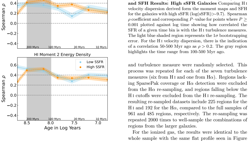
The central claim, stated most directly in the conclusions, is that the clearest correlation timescale is between star formation 100-500 Myr ago and the current HI energy surface density. At the 400 pc scale, Spearman rank correlations between HI energy surface density and SFR in the 100-200 Myr and 200-500 Myr bins reach $\rho \gtrsim 0.4$, with low $P$-values; restricting to regions with recent star formation sharpens the signal, with $\rho \simeq 0.52$ in the 100-200 Myr bin. The HI velocity dispersion correlates more weakly, and the correlation in the oldest, unresolved time bin is largely driven by a few high-mass, disturbed galaxies. The ionized gas, measured from H$\alpha$ line widths, shows no correlation at any probed timescale. A global analysis also shows HI turbulence correlated with star formation 100-300 Myr ago, alongside a milder 25-40 Myr signal consistent with an earlier study. The paper interprets this lag as the dissipation timescale of turbulence in the atomic interstellar medium, with $\tau_d = L_D / v_{\rm rms}$ linking the observed delay to the driving scale and velocity dispersion.

Load-bearing premise

The statistical tests treat each 400 pc region as an independent measurement, even though regions within a galaxy share gas, stars, and large-scale kinematics, and galaxies contribute very different numbers of regions, from 4 for Sextans B to 235 for IC 2574.

Editorial extensions

If this is right

Previous searches for a link between HI turbulence and recent star formation may have been looking at the wrong timescale; the relevant star formation happened roughly 100-500 Myr ago.
Supernovae can plausibly sustain HI turbulence with energy injection efficiencies of a few percent, resolving the apparent need for efficiencies near or above 100 percent found under short dissipation timescales.
The feedback timescale should vary with galaxy properties: higher specific star formation rates show shorter correlation lags, while lower-mass and lower-sSFR systems trend toward longer lags within the 100-500 Myr range.
Local and global turbulence timescales differ, so galaxy-wide averages mix regions with different driving scales and dissipation rates, which may explain the broader correlation window seen in the full sample.

Reading between the lines

Editorial extensions of the paper, not claims the author makes directly.

If the 100-500 Myr lag really is a dissipation timescale, then the same regional analysis applied to a single face-on dwarf with a measured disk scale-height gradient should show the lag increasing with radius, since $\tau_d = L_D / v_{\rm rms}$ grows with disk thickness; this radial prediction is left implicit in the paper.
The Spearman tests treat 400 pc regions as independent, but patches inside one galaxy share gas, stars, and large-scale kinematics, and galaxies contribute very unequal numbers of regions; a hierarchical model that accounts for within-galaxy clustering would test whether the 100-500 Myr signal survives at full significance.
If turbulence decays on ~100 Myr timescales, then stochastic variations in a galaxy's recent star formation history should imprint measurable scatter in HI energy density, and outliers such as the disturbed high-mass galaxies in this sample may be systems whose current turbulence still reflects an ancient burst.
The absence of an ionized-gas correlation may partly reflect the paper's insensitivity to the shortest timescales rather than a true physical decoupling, since H$\alpha$-based SFRs trace star formation within the last ~10 Myr, which the CMD-based SFHs cannot resolve.

Share X Bluesky LinkedIn Reddit HN

Editorial analysis

A structured set of objections, weighed in public.

Desk editor's note, referee report, and a circularity audit.

Desk Editor's Note

read the letter

Bottom line: the 100-500 Myr correlation between past star formation and HI energy surface density is probably real, but the paper overreaches when the abstract calls it a correlation with "atomic hydrogen turbulence measures." The velocity-dispersion correlations are much weaker than the energy-surface-density correlations, and since energy surface density is proportional to HI column density times sigma-squared, the headline result may be a gas-density correlation rather than a turbulence result.

What is genuinely new: the sample is 26 low-mass galaxies instead of the 5 in Papers I and II, with CMD-based SFHs and 400 pc HI kinematics. The H-alpha null is a useful negative result, honestly caveated by fiber coverage. The equal-region resampling test shows IC 2574 and other large galaxies are not carrying the signal by themselves. The mass and sSFR splits are sensible, and the authors are transparent about the influence of NGC 3738 and NGC 5253. No circular reasoning: the SFHs and turbulence measures come from independent data.

The soft spots are real but manageable. First, the Spearman tests treat roughly 961 regions as independent. Regions inside one galaxy share gas, stars, and large-scale kinematics, and the per-galaxy region counts range from 4 to 235. The P-values therefore overstate significance. The equal-region resampling fixes the galaxy-weighting problem, not spatial autocorrelation. A per-galaxy blocking or mixed model would be the right check.

Second, and more load-bearing: Sigma_E is proportional to M_HI/A_HI times sigma^2. The full-sample velocity-dispersion correlation is weak (rho = 0.26 at t > 500 Myr), and only after the young-star cut does sigma_central reach rho = 0.44 at 200-500 Myr. So the paper has not isolated the turbulent-velocity contribution from the column-density contribution. The conclusion that stellar feedback sustains HI turbulence on ~100 Myr timescales is supported only if the correlation survives when sigma is separated from column density. The abstract should say "HI energy surface density," not "turbulence measures."

Who this is for: observers and simulators working on feedback and HI turbulence in dwarfs. It deserves a serious referee, but the quantitative timescale claim needs to be softened and the autocorrelation issue addressed. I would send it to review with a request for those revisions, not desk-reject and not accept as is.

Referee Report

3 major / 8 minor

Summary. The paper combines CMD-derived star formation histories with VLA HI kinematics and WIYN SparsePak H-alpha kinematics for 26 low-mass galaxies, divided into 400 pc regions, to identify the lookback timescale over which stellar feedback correlates with present-day ISM turbulence. The central empirical result is that ionized gas velocity dispersion shows no correlation with star formation over 5-500 Myr, whereas HI energy surface density correlates most strongly with star formation 100-500 Myr ago (Spearman rho ~0.42-0.52 in the key bins). The authors interpret this as evidence that atomic gas turbulence is coupled to star formation on ~100 Myr timescales, consistent with a long turbulence dissipation timescale, and they contrast this with the shorter global timescale found in earlier work.

Significance. If the interpretation holds, the paper provides a direct observational constraint on the dissipation timescale of HI turbulence in low-mass galaxies and on the efficiency with which stellar feedback can sustain it. The sample is large and homogeneous, the SFH derivation is a well-established method, and the paper makes its regional SFH tables available as machine-readable products. The equal-region re-sampling test in Section 5.4 is a thoughtful robustness check, and the null result for H-alpha is reported honestly. The main risk is that the headline correlation is measured for HI energy surface density, which is proportional to HI column density, so the physical link to turbulence rather than gas content is not yet established.

major comments (3)

[Section 3.3, Eq. (5); Figures 6 and 8] The central correlation is between past star formation and Sigma_E,central = (3/2)(M_HI/A_HI)(1-f_wings)(1-f_cold) sigma_central^2, which is proportional to HI surface density. A correlation between past SFR and Sigma_E can therefore be produced entirely by spatial variations in gas column density, even if sigma_central is unrelated to star formation. The paper's own velocity-dispersion correlations are much weaker (rho=0.26 in the full sample at t>500 Myr, and rho=0.44 at 200-500 Myr only after the young-star cut), so the abstract's phrase 'atomic hydrogen turbulence measures' conflates energy surface density with turbulence. Please report partial Spearman correlations controlling for M_HI/A_HI, or equivalently show rank correlations separately for sigma and column density; without this, the physical interpretation that stellar feedback sustains HI turbulence on ~100 Myr timescales is not supported.
[Section 3.4 and Section 5.4] The Spearman tests treat the 961 regions as independent measurements, but regions within a galaxy share gas, stars, and large-scale kinematics, and the number of regions per galaxy ranges from 4 to 235. The equal-region re-sampling in Section 5.4 corrects for unequal galaxy weighting but does not remove intra-galaxy spatial autocorrelation, so the reported P-values likely overstate the significance of the correlations. A block bootstrap clustered by galaxy, or a mixed-effects model with galaxy as a random effect, would provide a more defensible significance statement. This is load-bearing because the sharpness of the 100-500 Myr timescale claim depends on the effective sample size.
[Section 5.1 and Section 8] The paper concludes that 'the clearest correlation timescale is between the SF 100-500 Myr ago and the current HI energy surface density,' but it does not formally test whether rho at 100-200 Myr and 200-500 Myr is significantly larger than rho at the younger time bins. The reported P-values are each against the null of no correlation, not against the null of equal correlation across bins. Since the time bins share the same gas measurements and adjacent SFH bins are correlated, a bootstrap or permutation test of the difference in Spearman coefficients should be added. Without such a test, the claimed preferred timescale is a descriptive statement rather than a statistically supported inference.

minor comments (8)

[Abstract] The phrase 'To investigate the timescales of turbulence low-mass galaxies' is missing the word 'in'; the abstract should also clarify that the 'atomic hydrogen turbulence measures' include both velocity dispersion and energy surface density, which the main text distinguishes.
[Section 4] The sentence 'Sections 5 an present the results' contains a typo and should read 'Sections 5 and 6 present the results.'
[Section 5.4] The sentence 'As a results larger galaxies, more distant galaxies, and those with multiple HST pointings contribute more regions' should be split or reworded; 'As a results' is a typo.
[Section 7.1] 'There effect becomes more significant when the number of regions per galaxy is equal' should read 'This effect becomes more significant...'.
[Table 8 note] The note ends with 'years ag and the error up and down' and should be 'years ago'; also the column-number descriptions appear off by one in several places and should be checked.
[Figure captions] Several captions contain 'Veloctiy' instead of 'Velocity' (e.g., Figures 5, 6, 8, 11) and '1σbootstrapping' is missing a space; these should be corrected.
[Section 3.4 vs Section 5.4] The bootstrap in Section 3.4 is described as 3000 resamples, while Section 5.4 uses 2000 resamples for the equal-region test; the text should clarify which resampling is shown in which figure.
[Appendix figure set] All appendix maps are labeled 'Figure 13' with different galaxy names; this is conventional for figure sets, but the captions should explicitly say 'Figure Set 13' so readers are not confused by the repeated number.

Circularity Check

0 steps flagged · score 0.0 of 10

No significant circularity: CMD-based SFHs and HI kinematics are independent measurements, and the dissipation-timescale comparison uses external relations.

full rationale

The central correlation is empirical and not circular. The SFHs are independently derived from CMD fitting with MATCH (Section 3.1), while the HI turbulence measures come from VLA kinematics and superprofile fitting (Section 3.3). The HI energy surface density is defined as Sigma_E = (3/2)(M_HI/A_HI)(1-f_wings)(1-f_cold) sigma_central^2, so the SFH is not an input to the turbulence measure by construction; the Spearman correlations in Figures 6-10 are measured relationships between two independent datasets. The dissipation-timescale discussion in Section 7.2 uses the external relation tau_d = L_D/v_rms from Bacchini et al. (2020a) and Mac Low (1999), with L_D taken from external scale-height measurements, and then compares the resulting 60-225 Myr range to the observed 100-200 Myr correlation as a consistency check rather than deriving the observed timescale from that relation. Self-citations to Paper I and Paper II are used for methodology and for reporting earlier timescale claims, but the present result is re-derived from a new 26-galaxy sample and does not assume the earlier timescale. The adopted cold-gas fraction f_cold = 0.15 comes from external literature (Stilp et al. 2013b; Young et al. 2003; Bolatto et al. 2011; Warren et al. 2012) and is a constant factor, so it cannot create a rank correlation. Concerns about the energy-surface-density measure conflating column density with turbulent velocity dispersion, and about treating regions as independent, are statistical and interpretational caveats rather than circular reasoning; even if the correlation were driven by M_HI/A_HI rather than sigma^2, it would still be an empirical correlation rather than an identity.

Assumptions & free parameters 6 free parameters · 6 assumptions · 0 invented entities

The central measurement is an empirical correlation, so it depends mainly on the fidelity of the SFH recovery and the HI turbulence measures. The listed parameters and assumptions are standard or clearly stated, and none is fitted to force the 100-500 Myr correlation. The main interpretive assumption is that the lagged correlation equals the dissipation timescale, which is plausible but not proven.

free parameters (6)

Region size = 400 pc per side
Fixed bin scale chosen to balance star counts, HI resolution, and feedback scales; the correlation timescale may depend on this choice, as discussed in Paper II.
f_cold (cold HI fraction) = 0.15
Adopted from Stilp et al. 2013b and prior dwarf galaxy estimates; used in Equation 5 to compute Sigma_E,central, not fitted here.
Turbulence driving scale L_D = 800 pc (assumed)
Assumed twice the disk scale height in Section 7.2 to estimate the dissipation timescale; not measured in this work.
sSFR division threshold = -9.7 log(yr^-1)
Hand-chosen boundary for high and low sSFR subsamples in Section 5.3; affects the sub-sample correlation results.
Mass bin boundaries = 7.7 and 8.7 log(M_sun)
Hand-chosen stellar mass bin edges in Section 5.3; affect the mass-dependence results.
Young star selection threshold = 50 young stars per region
Used in Section 5.2 to define the recently star-forming sample; adopted from Paper I.

assumptions (6)

domain assumption The IMF is Kroupa with 35% binary fraction and flat mass-ratio distribution
Assumed in MATCH synthetic CMDs in Section 3.1; affects recovered SFHs and hence the correlation timescale.
domain assumption Metallicity is non-decreasing with time and there is no internal differential extinction
These constraints reduce age-metallicity degeneracy but can bias recent SFHs if violated, as stated in Section 3.1.
domain assumption HI superprofiles are well described by a Gaussian core plus wings, with wings tracing low-density high-velocity gas
Underpins the definitions of sigma_central, f_wings, and sigma_wings used as turbulence measures in Section 3.3.
domain assumption HI velocity dispersion is isotropic, justifying the 3/2 prefactor in energy surface density
Used in Equations 4-6; if anisotropic, the derived energy densities are systematically biased.
domain assumption The correlation timescale equals the turbulence dissipation timescale tau_d = L_D / v_rms
Interpretive leap in Section 7.2, Equation 7; other processes such as SFH clustering or spatial transport could produce similar lagged correlations.
standard math Spearman correlation strength thresholds: |rho|<=0.2 no correlation, 0.2-0.4 weak, 0.4-0.7 strong
Standard but arbitrary thresholds used to classify correlation strengths in Section 3.4.

how reviews work

0 comments

Cite this review

Pith. "Pith review of Observed Timescales of Stellar Feedback in Star-Forming, Low-Mass Galaxies." pith.science (2026). https://pith.science/paper/VFNRPR2K

@misc{pith2026250719573,
  author       = {Pith},
  title        = {Pith review of: Observed Timescales of Stellar Feedback in Star-Forming, Low-Mass Galaxies},
  year         = {2026},
  howpublished = {\url{https://pith.science/paper/VFNRPR2K}},
  note         = {Machine review of arXiv:2507.19573}
}

abstract

Understanding the timescales of atomic gas turbulence is crucial to understanding the interplay between star formation and the interstellar medium (ISM). To investigate the timescales of turbulence low-mass galaxies ($10^{6.8}<M_\odot<10^9$), this study combines temporally resolved star formation histories (SFHs) -- derived from color-magnitude diagrams -- with kinematic data of the atomic and ionized hydrogen in a large sample of nearby, star-forming, low-mass galaxies. To best understand the timescales involved, SFHs and gas kinematics were analyzed in 400$\times$400 parsec regions to capture the local impacts of star formation. No strong correlation was found between the ionized gas velocity dispersion and the star formation activity over the past 5-500 Myr. In contrast, a consistent and significant correlation between the atomic hydrogen turbulence measures and the star formation activity t$\geq$100 Myr ago was identified. This correlation suggests the star formation activity and atomic gas are coupled on this timescale. This connection between star-formation activity $>$100 Myr ago, and the HI turbulence properties, may be related to the time scales over which turbulence decays in the ISM. Additionally, the results demonstrate a possible difference in the global and local turbulence properties of low-mass galaxies.

Figures

Figures reproduced from arXiv: 2507.19573 by the authors.

**Figure 1.** UGC 0685 Regions Maps Left: Two color image from HST F814W (red) and F606W (blue) observations with ACS, Center: H i dispersion map from VLA observations with isovelocity contours in 2.5 km s−1 step size, Right: σHα map from the SparsePak IFU on the WIYN 3.5m telescope, with each filled circle corresponding to a fiber’s size and position on the sky. Overlaid on all three panels are the outlines of the regions used f… view at source ↗

**Figure 2.** IC 2574 Regions Maps Left: Two color image from HST F814W (red) and F555W (blue) observations with ACS, Center: H i dispersion map from VLA observations with isovelocity contours in 2.5 km s−1 step size, Right: σHα map from the SparsePak IFU on the WIYN 3.5m telescope, with each filled circle corresponding to a fiber’s size and position on the sky. Overlaid on all three panels are the outlines of the regions used fo… view at source ↗

**Figure 3.** Example CMD’s Representative CMDs and SFHs for 400×400 pc regions in UGC 8201 and UGC 4459 . For both regions, the MS (blue), blue Helium burning stars (HeB) (green), and red HeB (red) sequences are traced. The SFHs have ≤25 Myr time resolution in the two most recent time bins with ∆log(t/yr)=0.3 time steps covering the 500 Myr baseline necessary for this projects scientific goals. The gray shading is the combined s… view at source ↗

Figures from the paper (34 more)

**Figure 4.** Figure 4: UGC 9240 Superprofile [PITH_FULL_IMAGE:figures/full_fig_p009_4.png]

**Figure 5.** Figure 5: Comparison of Hα derived ionized gas velocity dispersions and SFH results. Spearman ρ coefficient versus log time, which demonstrates how correlated the SFR of a given time bin is with the Hα FWHM for the whole sample. The light blue shaded region represents the 1σ b…

**Figure 6.** Figure 6: shows the correlation for all regions between the SFR in a each time bin and the velocity dispersion and H i energy surface density measured from the Gaussian superprofile fits. The light blue shaded region indicates the 1σ bootstrapping error from resampling the regi…

**Figure 7.** Figure 7: Comparison of σHI and SFR 500 Myr to 10 Gyr Ago: Full Spatial Coverage Sample and HighMass Sample. The H i velocity dispersion (σHI ) from the moment maps is plotted against the SFR averaged over 500 Myr to 10 Gyr for the Full Spatial Coverage Sample (Panel A) and for…

**Figure 9.** Figure 9: Comparison of ΣHI and SFH results for different mass samples. Comparing H i turbulence measures and SFH for the galaxies in different mass bins; galaxies with stellar masses 6.7 <M⋆ < 7.7 log(M⊙) in blue solid line, galaxies with stellar masses 7.7 <M⋆ < 8.7 log(M⊙) …

**Figure 11.** Figure 11: Comparison of H i Velocity Dispersion and SFH Results: High sSFR Galaxies Comparing H i velocity dispersion derived form the moment maps and SFH for the galaxies with high sSFR (log(sSFR)>-9.7). Spearman ρ coefficient and corresponding P–value for points where P ≥ 0.0…

**Figure 10.** Figure 10: Comparison of ΣHI and SFH Results: Binned sSFR Galaxies Comparing H i turbulence measures and SFH for the galaxies with low specific star formation rates FUV sSFR< −9.7 log(yr−1 , orange dashed line) and galaxies with high sSFR (log(sSFR)>-9.7, blue solid line). a) …

**Figure 12.** Figure 12: Comparison of Global H i Turbulence and SFH Results The median Spearman ρ coefficient and corresponding P value plotted against log time showing how correlated the SFR of a given time bin is with the H i turbulence measures. The light blue shaded region represents th…

**Figure 13.** Figure 13: UGC 0685 Maps Top Row UGC 0685 H i moment maps from VLA observations. Left: H i column density in 1021 hydrogen atoms cm−2 , Center: H i velocity map with isovelocity contours spaced every 10 km s−1 , Right: H i velocity dispersion map with isovelocity contours at 2.5…

**Figure 13.** Figure 13: NGC 0784 Top Row NGC0784 H i moment maps from VLA observations. Left: H i column density in 1021 hydrogen atoms cm−2 , Center: H i velocity map with isovelocity contours spaced every 10 km s−1 , Right: H i velocity dispersion map with isovelocity contours at 2.5 km s−…

**Figure 13.** Figure 13: NGC 2366 Top Row H i moment maps from VLA observations Left: H i column density in 1021 hydrogen atoms cm−2 , Center: H i velocity map with isovelocity contours spaces every 10 km s−1 , Right: H i velocity dispersion map with isovelocity contours at 2.5 km s−1 spacing…

**Figure 13.** Figure 13: Holmberg II Top Row H i moment maps from VLA observations. Left: H i column density in 1021 hydrogen atoms cm−2 , Center: H i velocity map with isovelocity contours spaced every 10 km s−1 , Right: H i velocity dispersion map with isovelocity contours at 1.5 km s−1 spa…

**Figure 13.** Figure 13: UGC 04459 Top Row H i moment maps from VLA observations. Left: H i column density in 1021 hydrogen atoms cm−2 , Center: H i velocity map with isovelocity contours spaced every 5 km s−1 , Right: H i velocity dispersion map with isovelocity contours at 2.5 km s−1 spacin…

**Figure 13.** Figure 13: Holmberg I Top Row Holmberg I H i moment maps from VLA observations. Left: H i column density in 1021 hydrogen atoms cm−2 , Center: H i velocity map with isovelocity contours spaced every 5 km s−1 , Right: H i velocity dispersion map with isovelocity contours at 2.5 k…

**Figure 13.** Figure 13: Sextans B Top Row H i moment maps from VLA observations. Left: H i column density in 1021 hydrogen atoms cm−2 , Center: H i velocity map with isovelocity contours spaced every 5 km s−1 , Right: H i velocity dispersion map with isovelocity contours at 1.5 km s−1 spacin…

**Figure 13.** Figure 13: Sextans A Top Row H i moment maps from VLA observations. Left: H i column density in 1021 hydrogen atoms cm−2 , Center: H i velocity map with isovelocity contours spaced every 5 km s−1 , Right: H i velocity dispersion map with isovelocity contours at 2.5 km s−1 spacin…

**Figure 13.** Figure 13: IC 2574 Top Row H i moment maps from VLA observations Left: H i column density in 1021 hydrogen atoms cm−2 , Center: H i velocity map with isovelocity contours spaces every 10 km s−1 , Right: H i velocity dispersion map with isovelocity contours at 2.5 km s−1 spacing.…

**Figure 13.** Figure 13: NGC 3738 Top Row H i moment maps from VLA observations. Left: H i column density in 1021 hydrogen atoms cm−2 , Center: H i velocity map with isovelocity contours spaced every 10 km s−1 , Right: H i velocity dispersion map with isovelocity contours at 5 km s−1 spacing.…

**Figure 13.** Figure 13: NGC 3741 Top Row H i moment maps from VLA observations. Left: H i column density in 1021 hydrogen atoms cm−2 , Center: H i velocity map with isovelocity contours spaced every 10 km s−1 , Right: H i velocity dispersion map with isovelocity contours at 1.5 km s−1 spacin…

**Figure 13.** Figure 13: NGC 4068 Top Row H i moment maps from VLA observations Left: H i column density in 1021 hydrogen atoms cm−2 , Center: H i velocity map with isovelocity contours spaces every 10 km s−1 , Right: H i velocity dispersion map with isovelocity contours at 2.5 km s−1 spacing…

**Figure 13.** Figure 13: NGC 4163 Top Row H i moment maps from VLA observations Left: H i column density in 1021 hydrogen atoms cm−2 , Center: H i velocity map with isovelocity contours spaces every 5 km s−1 , Right: H i velocity dispersion map with isovelocity contours at 2 km s−1 spacing. T…

**Figure 13.** Figure 13: NGC 4190 Top Row H i moment maps from VLA observations. Left: H i column density in 1021 hydrogen atoms cm−2 , Center: H i velocity map with isovelocity contours spaced every 10 km s−1 , Right: H i velocity dispersion map with isovelocity contours at 2.5 km s−1 spacin…

**Figure 13.** Figure 13: UGC 7577 Top Row hi moment maps from VLA observations. Left: H i column density in 1021 hydrogen atoms cm−2 , Center: H i velocity map with isovelocity contours spaced every 5 km s−1 , Right: H i velocity dispersion map with isovelocity contours at 1 km s−1 spacing. T…

**Figure 13.** Figure 13: UGCA 292 Top Row H i moment maps from VLA observations. Left: H i column density in 1021 hydrogen atoms cm−2 , Center: H i velocity map with isovelocity contours spaced every 5 km s−1 , Right: H i velocity dispersion map with isovelocity contours at 1 km s−1 spacing. …

**Figure 13.** Figure 13: UGC 8024 Top Row H i moment maps from VLA observations. Left: H i column density in 1021 hydrogen atoms cm−2 , Center: H i velocity map with isovelocity contours spaced every 10 km s−1 , Right: H i velocity dispersion map with isovelocity contours at 1.5 km s−1 spacin…

**Figure 13.** Figure 13: GR8 Top Row H i moment maps from VLA observations. Left: H i column density in 1021 hydrogen atoms cm−2 , Center: H i velocity map with isovelocity contours spaced every 5 km s−1 , Right: H i velocity dispersion map with isovelocity contours at 1.5 km s−1 spacing. The…

**Figure 13.** Figure 13: UGC 8201 Top Row H i moment maps from VLA observations. Left: H i column density in 1021 hydrogen atoms cm−2 , Center: H i velocity map with isovelocity contours spaced every 10 km s−1 , Right: H i velocity dispersion map with isovelocity contours at 2.5 km s−1 spacin…

**Figure 13.** Figure 13: NGC 5204 Top Row H i moment maps from VLA observations. Left: H i column density in 1021 hydrogen atoms cm−2 , Center: H i velocity map with isovelocity contours spaced every 10 km s−1 , Right: H i velocity dispersion map with isovelocity contours at 2.5 km s−1 spacin…

**Figure 13.** Figure 13: UGC 8638 Top Row H i moment maps from VLA observations. Left: H i column density in 1021 hydrogen atoms cm−2 , Center: H i velocity map with isovelocity contours spaced every 5 km s−1 , Right: H i velocity dispersion map with isovelocity contours at 1.5 km s−1 spacing…

**Figure 13.** Figure 13: UGC 8651 Top Row H i moment maps from VLA observations. Left: H i column density in 1021 hydrogen atoms cm−2 , Center: H i velocity map with isovelocity contours spaced every 5 km s−1 , Right: H i velocity dispersion map with isovelocity contours at 1 km s−1 spacing. …

**Figure 13.** Figure 13: NGC 5253 Top Row H i moment maps from VLA observations. Left: H i column density in 1021 hydrogen atoms cm−2 , Center: H i velocity map with isovelocity contours spaced every 10 km s−1 , Right: H i velocity dispersion map with isovelocity contours at 2.5 km s−1 spacin…

**Figure 13.** Figure 13: UGC 9128 Top Row H i moment maps from VLA observations Left: H i column density in 1021 hydrogen atoms cm−2 , Center: H i velocity map with isovelocity contours spaces every 5 km s−1 , Right: H i velocity dispersion map with isovelocity contours at 2.5 km s−1 spacing.…

**Figure 13.** Figure 13: UGC 9240 Top Row H i moment maps from VLA observations Left: H i column density in 1021 hydrogen atoms cm−2 , Center: H i velocity map with isovelocity contours spaces every 5 km s−1 , Right: H i velocity dispersion map with isovelocity contours at 2 km s−1 spacing. T…

**Figure 13.** Figure 13: NGC 6789 Top Row H i moment maps from VLA observations Left: H i column density in 1021 hydrogen atoms cm−2 , Center: H i velocity map with isovelocity contours spaces every 5 km s−1 , Right: H i velocity dispersion map with isovelocity contours at 2.5 km s−1 spacing.…

Discussion (0). Sign in to comment.

Reference graph

Works this paper leans on

25 extracted references · 18 canonical work pages

[1]

P., Tollerud, E

Astropy Collaboration, Robitaille, T. P., Tollerud, E. J., et al. 2013, A&A, 558, A33, doi: 10.1051/0004-6361/201322068 Astropy Collaboration, Price-Whelan, A. M., Sip˝ ocz, B. M., et al. 2018, AJ, 156, 123, doi: 10.3847/1538-3881/aabc4f Bacchini, C., Fraternali, F., Iorio, G., & Pezzulli, G. 2019, A&A, 622, A64, doi: 10.1051/0004-6361/201834382 Bacchini,...

arXiv 2000
[3]

NGC 2366 T op RowHimoment maps from VLA observations Left: Hicolumn density in 10 21 hydrogen atoms cm−2, Center: Hivelocity map with isovelocity contours spaces every 10 km s −1, Right: Hivelocity dispersion map with isovelocity contours at 2.5 km s−1 spacing. The beam size (22.89”×21.25”) of the Hidata cube used is shown in the bottom left of the left p...

work page 2000
[4]

Holmberg II T op RowHimoment maps from VLA observations. Left: Hicolumn density in 10 21 hydrogen atoms cm−2, Center: Hivelocity map with isovelocity contours spaced every 10 km s −1, Right: Hivelocity dispersion map with isovelocity contours at 1.5 km s −1 spacing. The beam size (10.73”×10.40”) of the Hidata cube used is shown in the bottom left of the l...

arXiv 2000
[5]

UGC 04459 T op RowHimoment maps from VLA observations. Left: Hicolumn density in 10 21 hydrogen atoms cm−2, Center: Hivelocity map with isovelocity contours spaced every 5 km s −1, Right: Hivelocity dispersion map with isovelocity contours at 2.5 km s−1 spacing. The beam size (19.65”×19.39”) of the Hidata cube used is shown in the bottom left of the left ...

arXiv 2000
[6]

Holmberg I T op Row Holmberg IHimoment maps from VLA observations. Left: Hicolumn density in 10 21 hydrogen atoms cm−2, Center: Hivelocity map with isovelocity contours spaced every 5 km s −1, Right: Hivelocity dispersion map with isovelocity contours at 2.5 km s −1 spacing. The beam size (9.77”×7.50”) of the Hidata cube used is shown in the bottom left o...

arXiv 2000
[7]

Sextans B T op RowHimoment maps from VLA observations. Left: Hicolumn density in 10 21 hydrogen atoms cm−2, Center: Hivelocity map with isovelocity contours spaced every 5 km s −1, Right: Hivelocity dispersion map with isovelocity contours at 1.5 km s −1 spacing. The beam size (21.26”×20.11”) of the Hidata cube used is shown in the bottom left of the left...

2000
[8]

Sextans A T op RowHimoment maps from VLA observations. Left: Hicolumn density in 10 21 hydrogen atoms cm−2, Center: Hivelocity map with isovelocity contours spaced every 5 km s −1, Right: Hivelocity dispersion map with isovelocity contours at 2.5 km s −1 spacing. The beam size (13.67”×10.68”) of the Hidata cube used is shown in the bottom left of the left...

arXiv 2000
[9]

IC 2574 T op RowHimoment maps from VLA observations Left: Hicolumn density in 10 21 hydrogen atoms cm−2, Center: Hivelocity map with isovelocity contours spaces every 10 km s −1, Right: Hivelocity dispersion map with isovelocity contours at 2.5 km s−1 spacing. The beam size (13.18”×12.45”) of the Hidata cube used is shown in the bottom left of the left pa...

2000

Show all 25 references

[10]

17'30" 00

NGC 3738 T op RowHimoment maps from VLA observations. Left: Hicolumn density in 10 21 hydrogen atoms cm−2, Center: Hivelocity map with isovelocity contours spaced every 10 km s −1, Right: Hivelocity dispersion map with isovelocity contours at 5 km s −1 spacing. The beam size (...

2000
[11]

NGC 3741 T op RowHimoment maps from VLA observations. Left: Hicolumn density in 10 21 hydrogen atoms cm−2, Center: Hivelocity map with isovelocity contours spaced every 10 km s −1, Right: Hivelocity dispersion map with isovelocity contours at 1.5 km s −1 spacing. The beam size...

2000
[12]

NGC 4068 T op RowHimoment maps from VLA observations Left: Hicolumn density in 10 21 hydrogen atoms cm−2, Center: Hivelocity map with isovelocity contours spaces every 10 km s −1, Right: Hivelocity dispersion map with isovelocity contours at 2.5 km s −1 spacing. The beam size ...

2000
[13]

NGC 0784 T op RowNGC0784 Himoment maps from VLA observations. Left: Hicolumn density in 10 21 hydrogen atoms cm−2, Center: Hivelocity map with isovelocity contours spaced every 10 km s −1, Right: Hivelocity dispersion map with isovelocity contours at 2.5 km s −1 spacing. The b...

2000
[14]

38'30" 00

NGC 4163 T op RowHimoment maps from VLA observations Left: Hicolumn density in 10 21 hydrogen atoms cm−2, Center: Hivelocity map with isovelocity contours spaces every 5 km s −1, Right: Hivelocity dispersion map with isovelocity contours at 2 km s −1 spacing. The beam size (15...

2000
[15]

NGC 4190 T op RowHimoment maps from VLA observations. Left: Hicolumn density in 10 21 hydrogen atoms cm−2, Center: Hivelocity map with isovelocity contours spaced every 10 km s −1, Right: Hivelocity dispersion map with isovelocity contours at 2.5 km s −1 spacing. The beam size...

2000
[16]

46'30" 00

UGC 7577 T op Rowhi moment maps from VLA observations. Left: Hicolumn density in 10 21 hydrogen atoms cm−2, Center: Hivelocity map with isovelocity contours spaced every 5 km s −1, Right: Hivelocity dispersion map with isovelocity contours at 1 km s −1 spacing. The beam size (...

2000
[17]

UGCA 292 T op RowHimoment maps from VLA observations. Left: Hicolumn density in 10 21 hydrogen atoms cm−2, Center: Hivelocity map with isovelocity contours spaced every 5 km s −1, Right: Hivelocity dispersion map with isovelocity contours at 1 km s −1 spacing. The beam size (1...

2000
[18]

UGC 8024 T op RowHimoment maps from VLA observations. Left: Hicolumn density in 10 21 hydrogen atoms cm−2, Center: Hivelocity map with isovelocity contours spaced every 10 km s −1, Right: Hivelocity dispersion map with isovelocity contours at 1.5 km s−1 spacing. The beam size ...

2000
[19]

GR8 T op RowHimoment maps from VLA observations. Left: Hicolumn density in 10 21 hydrogen atoms cm−2, Center: Hivelocity map with isovelocity contours spaced every 5 km s −1, Right: Hivelocity dispersion map with isovelocity contours at 1.5 km s −1 spacing. The beam size (17.4...

2000
[20]

25'30" 00

UGC 8201 T op RowHimoment maps from VLA observations. Left: Hicolumn density in 10 21 hydrogen atoms cm−2, Center: Hivelocity map with isovelocity contours spaced every 10 km s −1, Right: Hivelocity dispersion map with isovelocity contours at 2.5 km s−1 spacing. The beam size ...

2000
[21]

00" 46'30

NGC 5204 T op RowHimoment maps from VLA observations. Left: Hicolumn density in 10 21 hydrogen atoms cm−2, Center: Hivelocity map with isovelocity contours spaced every 10 km s −1, Right: Hivelocity dispersion map with isovelocity contours at 2.5 km s −1 spacing. The beam size...

2000
[22]

45'30" 00

UGC 8638 T op RowHimoment maps from VLA observations. Left: Hicolumn density in 10 21 hydrogen atoms cm−2, Center: Hivelocity map with isovelocity contours spaced every 5 km s −1, Right: Hivelocity dispersion map with isovelocity contours at 1.5 km s−1 spacing. The beam size (...

2000
[23]

UGC 8651 T op RowHimoment maps from VLA observations. Left: Hicolumn density in 10 21 hydrogen atoms cm−2, Center: Hivelocity map with isovelocity contours spaced every 5 km s −1, Right: Hivelocity dispersion map with isovelocity contours at 1 km s −1 spacing. The beam size (1...

2000
[24]

03'30" 00

NGC 5253 T op RowHimoment maps from VLA observations. Left: Hicolumn density in 10 21 hydrogen atoms cm−2, Center: Hivelocity map with isovelocity contours spaced every 10 km s −1, Right: Hivelocity dispersion map with isovelocity contours at 2.5 km s −1 spacing. The beam size...

2009
[25]

UGC 9128 T op RowHimoment maps from VLA observations Left: Hicolumn density in 10 21 hydrogen atoms cm−2, Center: Hivelocity map with isovelocity contours spaces every 5 km s −1, Right: Hivelocity dispersion map with isovelocity contours at 2.5 km s −1 spacing. The beam size (...

2000
[26]

58'30" 00

UGC 9240 T op RowHimoment maps from VLA observations Left: Hicolumn density in 10 21 hydrogen atoms cm−2, Center: Hivelocity map with isovelocity contours spaces every 5 km s −1, Right: Hivelocity dispersion map with isovelocity contours at 2 km s −1 spacing. The beam size (16...

2000

Pith tools

Reviewed August 6, 2026 · model on record in the stance chip above.

[1] [1]

P., Tollerud, E

Astropy Collaboration, Robitaille, T. P., Tollerud, E. J., et al. 2013, A&A, 558, A33, doi: 10.1051/0004-6361/201322068 Astropy Collaboration, Price-Whelan, A. M., Sip˝ ocz, B. M., et al. 2018, AJ, 156, 123, doi: 10.3847/1538-3881/aabc4f Bacchini, C., Fraternali, F., Iorio, G., & Pezzulli, G. 2019, A&A, 622, A64, doi: 10.1051/0004-6361/201834382 Bacchini,...

arXiv 2000

[2] [3]

NGC 2366 T op RowHimoment maps from VLA observations Left: Hicolumn density in 10 21 hydrogen atoms cm−2, Center: Hivelocity map with isovelocity contours spaces every 10 km s −1, Right: Hivelocity dispersion map with isovelocity contours at 2.5 km s−1 spacing. The beam size (22.89”×21.25”) of the Hidata cube used is shown in the bottom left of the left p...

work page 2000

[3] [4]

Holmberg II T op RowHimoment maps from VLA observations. Left: Hicolumn density in 10 21 hydrogen atoms cm−2, Center: Hivelocity map with isovelocity contours spaced every 10 km s −1, Right: Hivelocity dispersion map with isovelocity contours at 1.5 km s −1 spacing. The beam size (10.73”×10.40”) of the Hidata cube used is shown in the bottom left of the l...

arXiv 2000

[4] [5]

UGC 04459 T op RowHimoment maps from VLA observations. Left: Hicolumn density in 10 21 hydrogen atoms cm−2, Center: Hivelocity map with isovelocity contours spaced every 5 km s −1, Right: Hivelocity dispersion map with isovelocity contours at 2.5 km s−1 spacing. The beam size (19.65”×19.39”) of the Hidata cube used is shown in the bottom left of the left ...

arXiv 2000

[5] [6]

Holmberg I T op Row Holmberg IHimoment maps from VLA observations. Left: Hicolumn density in 10 21 hydrogen atoms cm−2, Center: Hivelocity map with isovelocity contours spaced every 5 km s −1, Right: Hivelocity dispersion map with isovelocity contours at 2.5 km s −1 spacing. The beam size (9.77”×7.50”) of the Hidata cube used is shown in the bottom left o...

arXiv 2000

[6] [7]

Sextans B T op RowHimoment maps from VLA observations. Left: Hicolumn density in 10 21 hydrogen atoms cm−2, Center: Hivelocity map with isovelocity contours spaced every 5 km s −1, Right: Hivelocity dispersion map with isovelocity contours at 1.5 km s −1 spacing. The beam size (21.26”×20.11”) of the Hidata cube used is shown in the bottom left of the left...

2000

[7] [8]

Sextans A T op RowHimoment maps from VLA observations. Left: Hicolumn density in 10 21 hydrogen atoms cm−2, Center: Hivelocity map with isovelocity contours spaced every 5 km s −1, Right: Hivelocity dispersion map with isovelocity contours at 2.5 km s −1 spacing. The beam size (13.67”×10.68”) of the Hidata cube used is shown in the bottom left of the left...

arXiv 2000

[8] [9]

IC 2574 T op RowHimoment maps from VLA observations Left: Hicolumn density in 10 21 hydrogen atoms cm−2, Center: Hivelocity map with isovelocity contours spaces every 10 km s −1, Right: Hivelocity dispersion map with isovelocity contours at 2.5 km s−1 spacing. The beam size (13.18”×12.45”) of the Hidata cube used is shown in the bottom left of the left pa...

2000