REVIEW 2 major objections 6 minor 29 references
A generalized optimal fourth-order finite difference scheme for a 2D Helmholtz equation with the perfectly matched layer boundary condition
T0 review · 2 major / 6 minor · reviewed 2026-08-14 · deepseek-v4-flash
Pith's one-line read The paper proves two point-weighting finite-difference stencils are fourth-order consistent with the Helmholtz equation with PML, fixing the earlier 17-point scheme's inconsistency.
desk verdict A genuinely new 17-point point-weighting stencil for Helmholtz-PML with solid interior convergence, but the PML consistency proof assumes smoothness the paper's own damping profile does not have. read the letter →
The pith
A machine-rendered reading of the paper's core claim, the machinery that carries it, and where it could break.
The reading
What carries the argument
The central mechanism is the point-weighting substitution: before applying the fourth-order difference operator, each off-center grid value is replaced by a weighted arithmetic average of neighboring values, with the weights required to sum to one. The 25-point scheme uses the substitutions in (12)-(13); the 17-point scheme uses (23)-(24). These substitutions preserve the $O(h^4)$ Taylor expansion of the operator while coupling the stencil in the transverse direction, which is what restores consistency for the PML equation and permits unequal spacings $\Delta x \neq \Delta z$. The mass term $k^2 C p$ is approximated by the operators $I^{(j)}$ with weights $c_j$ and $d_j$ that also sum to one. Least-squares minimization of the numerical-dispersion functional over propagation angle and grid-points-per-wavelength interval then fixes the free weights.
What would settle it
Run a convergence study for the refined point-weighting 17-point scheme on a manufactured solution with the wavefield supported inside the PML, where the damping profiles (2)-(3) are active; if the C-norm error over the layer does not shrink by roughly a factor of 16 when the grid is halved, the fourth-order claim fails exactly where the PML matters.
Extended reading notes
Core claim
On its own terms, the paper's discovery is that a fourth-order finite-difference discretization of the PML-modified Helmholtz equation can be made pointwise consistent by replacing individual grid values in the difference operator with weighted averages of neighboring values, and that this repairs the inconsistency of the authors' earlier 17-point scheme. The two resulting stencils, optimal point-weighting 25p and optimal point-weighting 17p, satisfy the Helmholtz-PML equation up to $O(h^4)$ error terms for essentially arbitrary weights, provided the relevant weights sum to one; the numerical wavenumber obeys $(k_N)^2 = k^2(1+O(k^6h^6))$. The authors present the 17-point version as a practical replacement for the inconsistent 17-point scheme, with a smaller matrix bandwidth and support for unequal spacings $\Delta x \neq \Delta z$.
Load-bearing premise
The fourth-order proof expands $p$ and the PML coefficients $A$, $B$, $C$ by Taylor's theorem at every grid point, so it assumes these fields are smooth everywhere, but the damping profiles used in the numerical examples are only piecewise smooth inside the PML.
Editorial extensions
If this is right
- The refined point-weighting 17-point scheme can be used in place of the earlier 17-point scheme for PML problems, keeping a narrower matrix bandwidth than the 25-point scheme while restoring consistency.
- Both stencils keep fourth-order accuracy when the step sizes in the two coordinate directions differ, removing the earlier 17-point scheme's restriction to equal spacing.
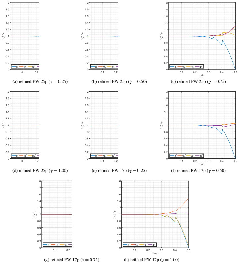
- With weights tuned on a given grid-point-per-wavelength interval, the schemes' normalized phase and group velocity curves stay close to one, so fewer grid points per wavelength are needed than with conventional second-order stencils.
- The wavenumber error relation $(k_N)^2 = k^2(1+O(k^6h^6))$ means the pollution error at fixed $kh$ is reduced by two orders relative to second-order schemes.
Reading between the lines
- Because the Taylor proof assumes smoothness of the PML coefficients, the observed order may drop to less than four inside the absorbing layer, where the damping profiles in (2)-(3) are only piecewise smooth; the paper does not report a separate convergence test restricted to the layer.
- The construction's parameter freedom suggests a natural stress test: fix the weights with the refined strategy on one velocity and frequency range, then evaluate the schemes outside that range, where the dispersion curves imply accuracy may degrade more sharply.
- The same point-weighting template should extend to three dimensions, as the authors list as future work, but the wider stencil and corner regions where both damping profiles vary will make the smoothness issue more pronounced.
Signed reviews
Editorial analysis
A structured set of objections, weighed in public.
Referee Report
Summary. The paper develops a point-weighting strategy for constructing fourth-order finite difference schemes for the two-dimensional Helmholtz equation with a perfectly matched layer (PML). Two schemes are proposed: an optimal point-weighting 25-point scheme and an optimal point-weighting 17-point scheme. Proposition 2.1 claims that both schemes are pointwise consistent with the Helmholtz-PML equation and are fourth-order accurate under only the sum constraints on the weighting parameters. A dispersion analysis is then used to select the free parameters by minimizing the numerical dispersion, giving the 'refined PW 25p' and 'refined PW 17p' schemes. Numerical experiments compare these schemes with existing rotated 9p, 17p, and 25p methods, and a layered-model example is used to argue that the new 17-point scheme removes the PML inconsistency of the earlier 17-point scheme of Dastour and Liao.
Significance. If the central claim is established, the refined 17-point scheme is a practically valuable contribution: it offers a narrower matrix bandwidth than the 25-point scheme while retaining fourth-order accuracy and PML consistency, which is important for large frequency-domain seismic modeling. The paper provides explicit stencils, dispersion relations, parameter-selection algorithms, and numerical comparisons, and the non-PML convergence experiments in Tables 1-4 show the expected roughly 16-fold error reduction on halving the mesh size. The main gap is that the consistency proof for the PML setting assumes more smoothness than the PML profile specified in the paper actually has, and the numerical examples do not provide a PML-specific convergence study. With that gap addressed, the contribution would justify publication.
major comments (2)
- [Section 2, Proposition 2.1 and Eqs. (33)-(39)] The Taylor-expansion proof of Proposition 2.1 assumes that p, A, B, and C are sufficiently smooth for the stated h^4 remainders to be controlled; Eqs. (37) and (39) contain derivatives of A and B up to order five and six (e.g., partial^5_x A and partial^6_x A). However, the PML damping profiles in Eqs. (2)-(3) are only C^1 at the interfaces l_x=0 and l_z=0, since the second derivative of sigma_x and sigma_z jumps from a nonzero value inside the layer to zero outside. Therefore A=sz/sx and B=sx/sz are not C^5 across the interface, and for any grid point whose 17-point or 25-point stencil includes points on both sides of a PML interface, the Taylor remainders in the proof are not bounded. Proposition 2.1 thus does not establish pointwise consistency or fourth-order accuracy in the PML setting that motivates the paper, unless the proof adds a smoothness hypothesis, treats interface-crossing stencils separately, or the PML profile is replaced by a smooth one.
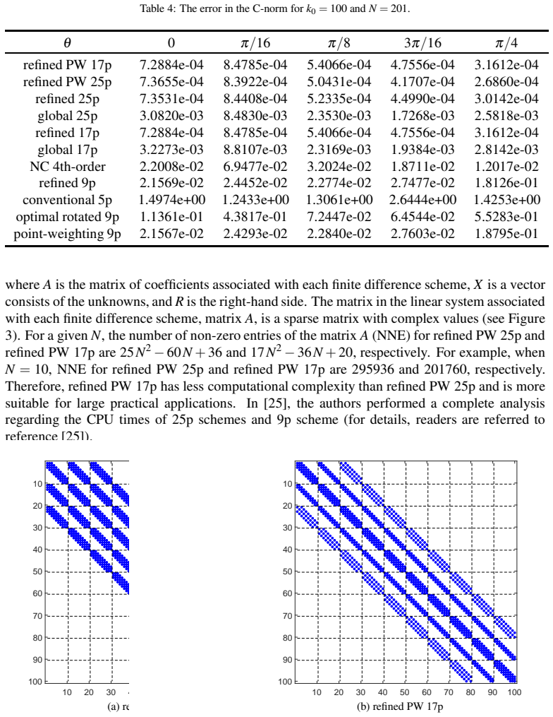
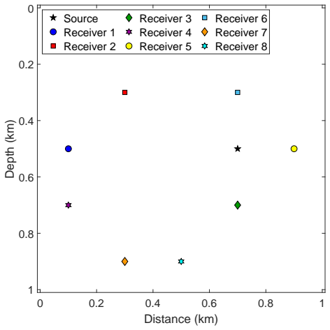
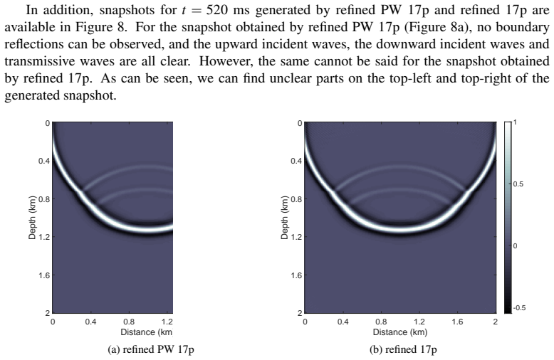
- [Section 4, Tables 1-4 and Examples 4.2-4.3] The numerical evidence does not yet fill the smoothness gap in the PML case. Example 4.1, which produces the convergence rates in Tables 1-4, uses Dirichlet boundary conditions with no PML, so the observed fourth-order error reduction does not test the PML claim. Example 4.2 uses a single grid size (nx=nz=51) with no refinement study, and Example 4.3 provides only qualitative wavefield snapshots. To support the central claim, the authors should report a convergence study for the Helmholtz-PML problem with the profile (2)-(3), for example by comparing against a known solution on a truncated domain with PML and measuring the C-norm error as h is halved.
minor comments (6)
- [Section 2, Eq. (6)] The fourth term on the right-hand side of Eq. (6) is evaluated at x_{m-3\Delta x/2}, but it should be x_{m+3\Delta x/2}; as written the formula is incorrect.
- [Section 2, Eq. (32) and Proposition 2.1 proof] The Taylor expansion for p^*_{m-2,n} in Eq. (32) uses b1 instead of a1; since this expansion is for the 25-point scheme, the coefficient should be a1.
- [Section 3, Eqs. (61) and (66)] The symbol 'g' appears in place of 'gamma' in several places, for example '(g4 + 1)' in Eq. (61) and '(g − 1)(g + 1)' in Eq. (66).
- [Section 3, Algorithm 2] The 'Result' line of Algorithm 2 says 'a1, . . . ,c4', but the algorithm solves for b1, d2, d3; this should be corrected.
- [Section 4.2] The sentence 'From [? ], the analytical solution of this homogeneous model is available' contains a missing citation placeholder; the reference should be supplied.
- [Section 2, after Eq. (42)] The discussion states that 'zeta and eta depend on k, A and B' where eta was previously defined as 1+1/gamma^2; the intended quantities are likely zeta and xi, the h^4 coefficients in Eqs. (41)-(42).
Circularity Check
No significant circularity: the consistency and fourth-order results are derived by direct Taylor expansion, the parameter optimization is explicit rather than disguised, and the numerical comparisons are external benchmarks.
full rationale
The paper's central derivation, Proposition 2.1, proves consistency and fourth-order accuracy for the point-weighting 25-point and 17-point schemes by expanding the stencil coefficients with Taylor's theorem and showing the truncation error is O(h^4) whenever the parameter normalization conditions hold. This is a direct mathematical derivation, not a restatement of an input or a fitted quantity. The later minimization of the numerical-dispersion functionals is explicitly presented as parameter selection by least squares, so the favorable dispersion curves and reduced phase errors in the examples are consequences of an announced optimization, not hidden fits renamed as predictions. The self-citations to the authors' prior work, especially [25], are used to motivate the new 17-point scheme and to explain why the older 17-point scheme is inconsistent in the PML; however, the new scheme's consistency proof does not depend on those results, so the self-citations are not load-bearing. The reviewer-flagged lack of smoothness of the PML damping profile is a legitimate correctness concern about the domain of validity of the Taylor-based proof, but it is not circularity: the proof would be invalid or incomplete in the PML region if the required derivatives do not exist, yet that does not make the claim equivalent to its inputs by construction. Because the central consistency and accuracy statements are derived from first principles and the parameter-fitting step is explicit and benchmarked against external exact solutions and existing schemes, the paper exhibits no significant circularity.
Assumptions & free parameters
free parameters (8)
- a1 (25p point-weighting parameter) =
not reported; solve least-squares system (76)
- b1 (17p point-weighting parameter) =
not reported; solve least-squares system (77)
- c2 (25p interpolation weight) =
not reported
- c3 (25p interpolation weight) =
not reported
- c4 (25p interpolation weight) =
not reported
- d2 (17p interpolation weight) =
not reported
- d3 (17p interpolation weight) =
not reported
- IG = [Gmin, Gmax] (optimization interval) =
fixed bands such as [2,2.5], [4,5], [10,400], or a priori intervals from Eq. (81)
assumptions (4)
- domain assumption Taylor's theorem and sufficient smoothness of p, A, B, C for the expansions in Proposition 2.1
- domain assumption PML damping profiles from Eqs. (2)-(3) with a0 = 1.79 taken from [26]
- domain assumption Infinite homogeneous medium with plane wave solution for dispersion analysis
- standard math Least-squares solution of the overdetermined systems (76) and (77) yields parameters that minimize J* and J-tilde
Cite this review
Pith. "Pith review of A generalized optimal fourth-order finite difference scheme for a 2D Helmholtz equation with the perfectly matched layer boundary condition." pith.science (2026). https://pith.science/paper/VRX7LB2U
@misc{pith2026190807403,
  author       = {Pith},
  title        = {Pith review of: A generalized optimal fourth-order finite difference scheme for a 2D Helmholtz equation with the perfectly matched layer boundary condition},
  year         = {2026},
  howpublished = {\url{https://pith.science/paper/VRX7LB2U}},
  note         = {Machine review of arXiv:1908.07403}
}
read the original abstract
A crucial part of successful wave propagation related inverse problems is an efficient and accurate numerical scheme for solving the seismic wave equations. In particular, the numerical solution to a multi-dimensional Helmholtz equation can be troublesome when the perfectly matched layer (PML) boundary condition is implemented. In this paper, we present a general approach for constructing fourth-order finite difference schemes for the Helmholtz equation with PML in the two-dimensional domain based on point-weighting strategy. Particularly, we develop two optimal fourth-order finite difference schemes, optimal point-weighting 25p and optimal point-weighting 17p. It is shown that the two schemes are consistent with the Helmholtz equation with PML. Moreover, an error analysis for the numerical approximation of the exact wavenumber is provided. Based on minimizing the numerical dispersion, we implement the refined choice strategy for selecting optimal parameters and present refined point-weighting 25p and refined point-weighting 17p finite difference schemes. Furthermore, three numerical examples are provided to illustrate the accuracy and effectiveness of the new methods in reducing numerical dispersion.
Figures

Figures from the paper (6 more)



Reference graph
Works this paper leans on
-
[25]
H. Dastour, W. Liao, A fourth-order optimal finite diffe rence scheme for the helmholtz equation with pml, Com- puters & Mathematics with Applications 6 (78) (2009) 2147–2 165
work page 2009
-
[1]
B. Hustedt, S. Operto, J. Virieux, Mixed-grid and stagge red-grid finite-difference methods for frequency-domain acoustic wave modelling, Geophysical Journal Internation al 157 (3) (2004) 1269–1296
work page 2004
-
[2]
T. Wu, A dispersion minimizing compact finite difference scheme for the 2d helmholtz equation, Journal of Com- putational and Applied Mathematics 311 (2017) 497–512
work page 2017
-
[3]
F. Ihlenburg, I. Babuˇ ska, Dispersion analysis and erro r estimation of galerkin finite element methods for the helmholtz equation, International journal for numerical m ethods in engineering 38 (22) (1995) 3745–3774
work page 1995
-
[4]
F. Ihlenburg, I. Babuˇ ska, Finite element solution of th e helmholtz equation with high wave number part i: The h-version of the fem, Computers & Mathematics with Applicat ions 30 (9) (1995) 9–37
work page 1995
-
[5]
C.-H. Jo, C. Shin, J. H. Suh, An optimal 9-point, finite-di fference, frequency-space, 2-d scalar wave extrapolator, Geophysics 61 (2) (1996) 529–537
work page 1996
-
[6]
Z. Chen, D. Cheng, W. Feng, T. Wu, An optimal 9-point finite difference scheme for the helmholtz equation with pml., International Journal of Numerical Analysis & Modeli ng 10 (2) (2013)
work page 2013
-
[7]
C. Shin, H. Sohn, A frequency-space 2-d scalar wave extra polator using extended 25-point finite-difference opera- tor, Geophysics 63 (1) (1998) 289–296
work page 1998
Show all 29 references
-
[8]
Z. Chen, D. Cheng, T. Wu, A dispersion minimizing finite di fference scheme and preconditioned solver for the 3d helmholtz equation, Journal of Computational Physics 231 ( 24) (2012) 8152–8175. 31
2012
-
[9]
R. G. Pratt, M. Worthington, Inverse theory applied to mu lti-source cross-hole tomography. part 1: Acoustic wave- equation method, Geophysical prospecting 38 (3) (1990) 287 –310
1990
-
[10]
P . M. De Zeeuw, Matrix-dependent prolongations and res trictions in a blackbox multigrid solver, Journal of com- putational and applied mathematics 33 (1) (1990) 1–27
1990
-
[11]
Y . A. Erlangga, C. W. Oosterlee, C. Vuik, A novel multigr id based preconditioner for heterogeneous helmholtz problems, SIAM Journal on Scientific Computing 27 (4) (2006) 1471–1492
2006
-
[12]
M. B. van Gijzen, Y . A. Erlangga, C. Vuik, Spectral analy sis of the discrete helmholtz operator preconditioned with a shifted laplacian, SIAM Journal on Scientific Computing 29 (5) (2007) 1942–1958
2007
-
[13]
Chen, A generalized optimal 9-point scheme for fr equency-domain scalar wave equation, Journal of Applied Geophysics 92 (2013) 1–7
J.-B. Chen, A generalized optimal 9-point scheme for fr equency-domain scalar wave equation, Journal of Applied Geophysics 92 (2013) 1–7
2013
-
[14]
Collino, P
F. Collino, P . B. Monk, Optimizing the perfectly matche d layer, Computer methods in applied mechanics and engineering 164 (1-2) (1998) 157–171
1998
-
[15]
Berenger, A perfectly matched layer for the absor ption of electromagnetic waves, Journal of computational physics 114 (2) (1994) 185–200
J.-P . Berenger, A perfectly matched layer for the absor ption of electromagnetic waves, Journal of computational physics 114 (2) (1994) 185–200
1994
-
[16]
Turkel, A
E. Turkel, A. Y efet, Absorbing pml boundary layers for w ave-like equations, Applied Numerical Mathematics 27 (4) (1998) 533–557
1998
-
[17]
Singer, E
I. Singer, E. Turkel, A perfectly matched layer for the h elmholtz equation in a semi-infinite strip, Journal of Com- putational Physics 201 (2) (2004) 439–465
2004
-
[18]
Cheng, X
D. Cheng, X. Tan, T. Zeng, A dispersion minimizing finite difference scheme for the helmholtz equation based on point-weighting, Computers & Mathematics with Applicatio ns 73 (11) (2017) 2345–2359
2017
-
[19]
Harari, E
I. Harari, E. Turkel, Accurate finite difference method s for time-harmonic wave propagation, Journal of Computa- tional Physics 119 (2) (1995) 252–270
1995
-
[20]
Singer, E
I. Singer, E. Turkel, High-order finite difference meth ods for the helmholtz equation, Computer Methods in Applied Mechanics and Engineering 163 (1-4) (1998) 343–358
1998
-
[21]
Britt, S
S. Britt, S. Tsynkov, E. Turkel, Numerical simulation o f time-harmonic waves in inhomogeneous media using compact high order schemes, Communications in Computation al Physics 9 (3) (2011) 520–541
2011
-
[22]
Sutmann, Compact finite difference schemes of sixth o rder for the helmholtz equation, Journal of Computational and Applied Mathematics 203 (1) (2007) 15–31
G. Sutmann, Compact finite difference schemes of sixth o rder for the helmholtz equation, Journal of Computational and Applied Mathematics 203 (1) (2007) 15–31
2007
-
[23]
T. Wu, R. Xu, An optimal compact sixth-order finite diffe rence scheme for the helmholtz equation, Computers & Mathematics with Applications 75 (7) (2018) 2520–2537
2018
-
[24]
Turkel, D
E. Turkel, D. Gordon, R. Gordon, S. Tsynkov, Compact 2d a nd 3d sixth order schemes for the helmholtz equation with variable wave number, Journal of Computational Physic s 232 (1) (2013) 272–287
2013
-
[26]
Y . Zeng, J. He, Q. Liu, The application of the perfectly m atched layer in numerical modeling of wave propagation in poroelastic media, Geophysics 66 (4) (2001) 1258–1266
2001
-
[27]
L. N. Trefethen, Group velocity in finite difference sch emes, SIAM review 24 (2) (1982) 113–136
1982
-
[28]
T. A. Davis, I. S. Duff, An unsymmetric-pattern multifr ontal method for sparse lu factorization, SIAM Journal on Matrix Analysis and Applications 18 (1) (1997) 140–158
1997
-
[29]
T. A. Davis, Algorithm 832: Umfpack v4. 3—an unsymmetri c-pattern multifrontal method, ACM Transactions on Mathematical Software (TOMS) 30 (2) (2004) 196–199. 32
2004
Reviewed August 14, 2026 · model on record in the stance chip above.
Discussion (0). Continue with ORCID to comment.