REVIEW 3 major objections 5 minor 1 cited by
BASIL: Fast broadband line-rich spectral-cube fitting and image visualization via Bayesian quadrature
T0 review · 3 major / 5 minor · reviewed 2026-08-06 · deepseek-v4-flash
Pith's one-line read A 2-million-hour mapping job done in 180 hours
desk verdict A serious methods contribution for fast spectral-cube fitting, where the full pipeline is only validated on smooth Gaussian maps and the more realistic benchmark tests only the map-reconstruction block, leaving the headline speed claim for complex sources open. read the letter →
The pith
A machine-rendered reading of the paper's core claim, the machinery that carries it, and where it could break.
The reading
What carries the argument
The load-bearing mechanism is the reformulation of parallel active-learning pixel selection as a Bayesian quadrature problem: the GP's predictive variance is treated as an unnormalized target distribution, and kernel quadrature picks a batch of points that best represents that distribution, effectively maximizing the reduction in integrated uncertainty across the map. The argument also relies on a Kronecker-structured multi-output Gaussian process that shares information across the 468 parameter maps, and on stochastic variational inference with a mixture likelihood that treats channels contaminated by unidentified lines as outliers.
What would settle it
Run the full BASIL pipeline on a realistic spectral cube with known ground-truth maps that contain sharp chemical boundaries, and check whether the GP-reconstructed maps reproduce those edges: if deviations at the boundaries exceed the roughly ten percent mean square error reported on the Gaussian benchmark maps, the smoothness assumption is violated.
Extended reading notes
Core claim
The central claim is that molecular parameter maps can be estimated without exhaustively fitting every pixel. The pipeline works in two stages: stochastic variational inference estimates the four LTE parameters per molecule at individual positions, and a multi-output Gaussian process then extrapolates those estimates over the spatial domain, greedily querying the pixels with the highest predictive variance through the batch Bayesian active learning method BASQ. In the synthetic benchmark of 117 molecules, each with excitation temperature, column density, centroid velocity, and line width, roughly 1,000 queried locations suffice to produce maps whose errors are comparable to full pixel-by-pixel fitting, while the compute time drops from an estimated two million hours to about 180 hours. The paper attributes the speed to sublinear convergence of the GP prediction error, and emphasizes that the framework simultaneously fits all molecules under a one-component LTE model to handle line blending.
Load-bearing premise
The Gaussian process assumes the true parameter maps are smooth with a stationary correlation length, so sharp boundaries, sub-beam structure, or nonstationary emission in real sources would be smoothed away and the demonstrated speed-accuracy trade-off would degrade.
Editorial extensions
If this is right
- Any wideband spectral cube of a line-rich source can be mapped at a fraction of the compute, with the same pixel-selection and GP recipe reusable for other per-pixel fitting problems.
- Systematic analyses of large surveys become feasible, enabling unbiased statistics of chemical abundances and kinematics across many hot cores and hot corinos rather than case studies.
- The iterative workflow provides a natural quick-look mode: about 20 hours yields visually reliable maps, and continued iterations refine them, matching the data volume of next-generation ALMA observations.
- The dense, continuous maps produced by the GP remove the jagged, pixel-to-pixel discontinuities that plague independent per-pixel optimizations.
- The estimated two-million-hour MCMC baseline makes the speed gain concrete: the reported 180 hours is roughly four orders of magnitude faster under the paper's assumptions.
Reading between the lines
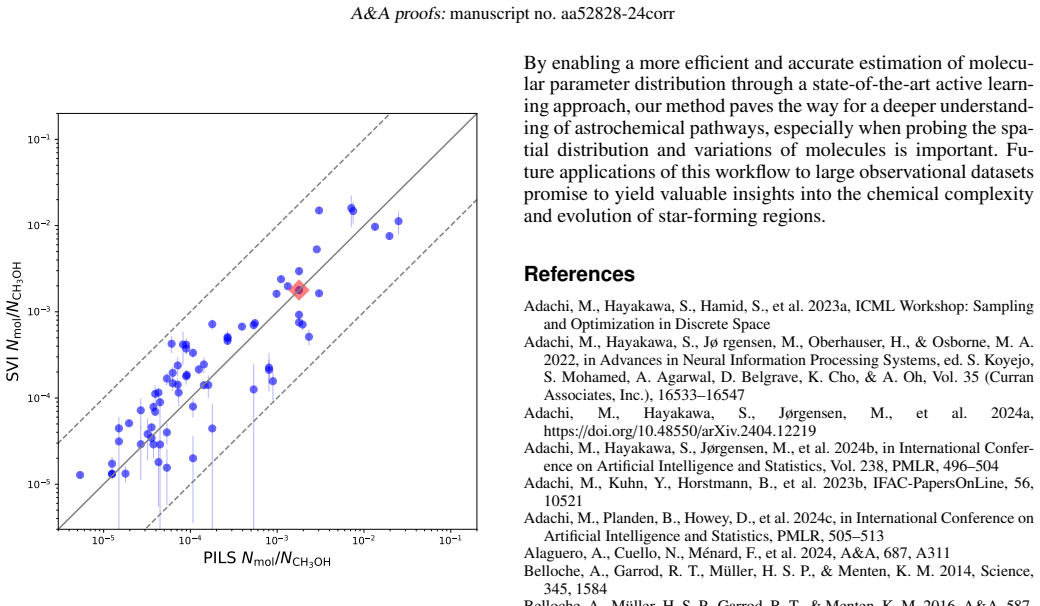
- A direct test of the full pipeline would apply it to an observed datacube, such as the PILS data toward IRAS16293B, and compare the GP-produced maps against published column densities; the paper only validates the SVI step against those data, not the GP and BASQ extrapolation.
- The smoothness assumption limits the method on sources with sharp chemical boundaries or sub-beam structure; using nonstationary or spatially varying kernels is a natural next step the paper does not test.
- The framework is not specific to LTE or molecular line fitting; it could accelerate any spectral-cube analysis where the underlying parameter fields are spatially smooth, such as line decomposition in Galactic plane surveys.
- Because the benchmark maps were generated as two-component Gaussians, the reported error rates may be optimistic; realistic emission with spiral-arm-like structure (as in the appendix test) would be a fairer measure of the full pipeline.
Editorial analysis
A structured set of objections, weighed in public.
Referee Report
Summary. The paper presents BASIL, a workflow that combines stochastic variational inference (SVI) for per-pixel LTE spectral fitting with Gaussian-process-based Bayesian active learning (BASQ) to estimate molecular parameter maps from line-rich spectral datacubes. The method is benchmarked on a synthetic 200x200-pixel cube with 117 molecules and 138,016 frequency channels, claiming 468 parameter maps in about 180 hours, visually reliable maps after about 20 hours, and an RMSE comparable to ground truth while being orders of magnitude faster than pixel-by-pixel MCMC. The SVI step is additionally cross-validated against published PILS column densities.
Significance. If the headline claims hold, BASIL would be a practically valuable tool for the large wideband surveys expected from the ALMA Wideband Sensitivity Upgrade. The paper's strengths include a public code repository with a minimal working example, a synthetic benchmark with known ground truth, the use of a realistic hydrodynamical simulation in Appendix B for the map-reconstruction step, and a comparison of SVI-derived column densities against PILS results. The central methodological idea—replacing exhaustive pixel-by-pixel fitting with active learning over a GP surrogate—is sensible and the separation of the SVI and BASQ blocks is clearly described. However, the validation as presented supports the conclusion only under favorable smoothness assumptions, and some of the abstract-level claims go beyond what the experiments directly demonstrate.
major comments (3)
- [§6.1, Appendix B] The full-pipeline benchmark in §6.1 uses synthetic parameter maps generated as two-component multivariate normals, which is the ideal case for an RBF-kernel GP. Appendix B tests the BASQ/GP block on the more realistic V892 Tau simulation maps, but it isolates that block by replacing actual SVI outputs with ground-truth maps plus i.i.d. noise; no full-pipeline wall-clock time or RMSE including SVI error is reported. The paper itself states in §6.1 that the universal approximation property does not imply sample efficiency at the n≈1000 scale used here. Because the headline speed-accuracy trade-off depends on reconstructing 468 maps from roughly 1000 SVI-fitted pixels, the authors should run the full BASIL pipeline on non-smooth or simulated hot-core maps—for example, by feeding the V892 Tau maps through the actual LTE+SVI step—and report the resulting RMSE and time. Without such a test, the central claim is only demonstrated for maps that are essentially GP-friendly.
- [§4.1, Eqs. (8)–(9), §6.2] Equation (8) defines the RMSE as sqrt(mean(rSVI + rGP)), but the true squared error between the ground-truth map and the GP prediction is (y* - \hat f)^2 = rSVI + rGP + 2(y* - \hat y)(\hat y - \hat f). The cross term is omitted unless the SVI error and the GP error are uncorrelated, which is not established. Equation (9) further assumes the SVI estimation error is zero-mean Gaussian, yet §6.2 documents severe degeneracies for HNCO, HN13CO, and CH3COOH, with larger scatter in the low-Tex regime, so the zero-mean and Gaussianity assumptions are not obviously satisfied. Since Eq. (9) and the predictive-variance proxy in Eq. (10) are used for the stopping criterion and for uncertainty estimates on real data, the paper needs to justify or correct this decomposition and to assess the impact of biased or non-Gaussian SVI errors on both the GP surrogate and the active-learning acquisition.
- [Abstract, §6.3] The headline claim of being 'orders of magnitude faster' than traditional pixel-by-pixel MCMC rests on an unmeasured estimate of roughly 2e6 hours for the MCMC baseline, and the 'comparable RMSE' is not directly benchmarked against an MCMC fit; the synthetic experiments compare GP predictions with ground truth, not with MCMC results. The only measured comparison in §6.3 is the factor of about 50 relative to exhaustive SVI fitting (40,000 versus 1,000 queried locations). The authors should either provide the basis for the MCMC runtime estimate—including per-pixel runtime, number of walkers, burn-in, thinning, and convergence criteria—or reframe the speed and accuracy claims in terms of the measured SVI exhaustive-fit baseline.
minor comments (5)
- [§6.3] The statement that 'MSE values fall within the model prediction standard deviations and are approximately 10% of the ground-truth values' is ambiguous; the figures suggest the MSE is about 10% of the parameter range rather than 10% of the local ground-truth value, and this should be stated precisely.
- [Figure 9 caption] The caption says the MSE color scale is capped at 0.5 times the maximum model standard deviation, which is a nonstandard display choice; please clarify how this affects the visual impression of the MSE maps and whether the same cap is applied to all molecules.
- [§6.1] The removal of molecules with fewer than three transitions is an ad hoc cut that affects the claimed molecule count and the difficulty of the fitting problem; the paper should justify why three transitions is sufficient to constrain Nmol and Tex and state how many of the 117 entries are affected.
- [§5.2] The mixture likelihood for handling unidentified lines introduces an outlier probability as an additional optimized parameter, but the chosen prior or allowed range for this probability is not specified; adding this information would improve reproducibility.
- [Appendix B] The RMSE comparison in Figure B.2 appears to come from a single run; multiple random seeds or confidence intervals would strengthen the claim that BASQ outperforms random nearest-neighbor interpolation by a stable margin.
Circularity Check
No significant circularity: the central accuracy and speed claims are benchmarked against external synthetic ground truth; the only self-citation (BASQ convergence theorem) is not load-bearing.
full rationale
The paper's derivation chain is self-contained with respect to its accuracy claims. The GP is trained on SVI-inferred parameters and evaluated against externally generated ground-truth maps in Section 6 (synthetic datacube), not against quantities the GP itself produces by construction; Eq. (8) separates SVI error from GP error, and the reported MSE is computed against ground truths. The Appendix B benchmark, while isolating the GP+BASQ block and simulating SVI outputs as ground truth plus i.i.d. noise, is an honest partial test rather than a disguised prediction: the noisy values are external inputs, and the RMSE is measured against independent simulation maps. The claim of sublinear/exponential convergence relies on a published theorem from the authors' prior work (Adachi et al. 2022, Theorem 1), cited in Section 5.3; this is a self-citation, but it is not load-bearing because the empirical speedup is demonstrated on the synthetic cube and the theorem is a parameter-free mathematical result with its own proof. The main caveats are validity risks rather than circularity. Section 6.1 generates the benchmark maps as two-component multivariate normals, which are well matched to an RBF-kernel GP, and it explicitly warns that RBF universal approximation 'does not imply that the RBF kernel always provides better sample efficiency for function approximation compared to other kernels in practice.' Appendix B tests only the map-reconstruction block by adding i.i.d. noise to ground-truth maps, so it does not capture spatially correlated SVI bias or full-pipeline wall-clock. These concerns weaken external generalizability to non-smooth real hot-core maps, but no claimed result reduces to its own inputs by construction, and no fitted parameter is renamed as a prediction.
Assumptions & free parameters
free parameters (5)
- GP kernel hyperparameters (RBF lengthscale, output scale, noise variance) =
not reported in text
- SVI variational parameters (multivariate normal guide mean and covariance per pixel) =
not reported in text
- Batch size n =
50
- Outlier probability in the mixture likelihood =
not reported in text
- Synthetic ground-truth map parameters (peak centers and variances of two Gaussian components) =
drawn randomly per molecule
assumptions (7)
- domain assumption Local thermodynamic equilibrium with a single excitation temperature holds for all 117 molecules in hot cores and hot corinos.
- domain assumption Line optical depths from different molecules simply add, and radiative coupling between blended species is neglected.
- domain assumption Continuum-subtracted data are described by Tbg = 2.73 K, Tslope = 0, and tau_dust = 0.
- ad hoc to paper The SVI estimation error is zero-mean Gaussian, so the GP predictive variance is a valid proxy for the total RMSE.
- domain assumption Parameter maps are smooth enough for GP interpolation, and the chosen RBF kernel has sufficient capacity.
- domain assumption Molecular constants from CDMS, JPL, and LSD are accurate for all entries used.
- ad hoc to paper Molecules with fewer than three transitions in the frequency band can be removed from the fit.
Cite this review
Pith. "Pith review of BASIL: Fast broadband line-rich spectral-cube fitting and image visualization via Bayesian quadrature." pith.science (2026). https://pith.science/paper/WAEOO6ID
@misc{pith2026250623269,
  author       = {Pith},
  title        = {Pith review of: BASIL: Fast broadband line-rich spectral-cube fitting and image visualization via Bayesian quadrature},
  year         = {2026},
  howpublished = {\url{https://pith.science/paper/WAEOO6ID}},
  note         = {Machine review of arXiv:2506.23269}
}
read the original abstract
Mapping the spatial distributions and abundances of complex organic molecules in hot cores and hot corinos is crucial for understanding the astrochemical pathways and the inheritance of prebiotic material by nascent planetary systems. However, the line-rich spectra from these sources pose significant challenges for robustly fitting molecular parameters due to severe line blending and unidentified lines. We present an efficient framework, Bayesian Active Spectral-cube Inference and Learning (BASIL), for estimating molecular parameter maps for hundreds of molecules based on the local thermodynamic equilibrium (LTE) model, applied to wideband spectral datacubes of line-rich sources. We adopted stochastic variational inference to infer molecular parameters from spectra at individual positions, balancing between fitting accuracy and computational speed. For obtaining parameter maps, instead of querying every location or pixel, we introduced an active learning framework based on Bayesian quadrature and its parallelization. Specifically, we assessed and selected the locations or pixels of spectrum that are most informative for estimating the entire set of parameter maps by training a Gaussian processes model. By greedily selecting locations with maximum information gain, we achieve sublinear convergence. We benchmarked BASIL on a large synthetic datacube and demonstrated that it produces accurate 468 molecular parameter maps from 117 molecules within ~180 hours, orders of magnitude faster than traditional pixel-by-pixel fitting using Markov chain Monte Carlo methods, with visually reliable results emerging in just ~20 hours. Additional training iterations provide progressively more accurate results. This quick visualization meets the demands of big data in modern astronomical surveys.
Figures


Figures from the paper (7 more)


Forward citations
Cited by 1 Pith paper
-
End-to-end differentiable retrieval of molecular spectra using hydrodynamics, chemistry, and radiative transfer
An end-to-end differentiable JAX pipeline couples 1D hydrodynamics, time-dependent chemistry, and radiative transfer, and recovers shock and rate parameters from synthetic HCO+ spectra.
Reference graph
Works this paper leans on
-
[1]
2023 a , ICML Workshop: Sampling and Optimization in Discrete Space
Adachi, M., Hayakawa, S., Hamid, S., et al. 2023 a , ICML Workshop: Sampling and Optimization in Discrete Space
2023
-
[2]
Adachi, M., Hayakawa, S., J rgensen, M., Oberhauser, H., & Osborne, M. A. 2022, in Advances in Neural Information Processing Systems, ed. S. Koyejo, S. Mohamed, A. Agarwal, D. Belgrave, K. Cho, & A. Oh, Vol. 35 (Curran Associates, Inc.), 16533--16547
2022
-
[3]
2024 a , https://doi.org/10.48550/arXiv.2404.12219
Adachi, M., Hayakawa, S., J rgensen, M., et al. 2024 a , https://doi.org/10.48550/arXiv.2404.12219
-
[4]
2024 b , in International Conference on Artificial Intelligence and Statistics, Vol
Adachi, M., Hayakawa, S., J rgensen, M., et al. 2024 b , in International Conference on Artificial Intelligence and Statistics, Vol. 238, PMLR, 496--504
2024
-
[5]
2023 b , IFAC-PapersOnLine, 56, 10521
Adachi, M., Kuhn, Y., Horstmann, B., et al. 2023 b , IFAC-PapersOnLine, 56, 10521
2023
-
[6]
2024 c , in International Conference on Artificial Intelligence and Statistics, PMLR, 505--513
Adachi, M., Planden, B., Howey, D., et al. 2024 c , in International Conference on Artificial Intelligence and Statistics, PMLR, 505--513
2024
-
[7]
2024, , 687, A311
Alaguero , A., Cuello , N., M \'e nard , F., et al. 2024, , 687, A311
2024
-
[8]
T., M \"u ller , H
Belloche , A., Garrod , R. T., M \"u ller , H. S. P., & Menten , K. M. 2014, Science, 345, 1584
2014
Show all 98 references
-
[9]
Belloche , A., M \"u ller , H. S. P., Garrod , R. T., & Menten , K. M. 2016, , 587, A91
2016
-
[10]
Belloche , A., M \"u ller , H. S. P., Menten , K. M., Schilke , P., & Comito , C. 2013, , 559, A47
2013
-
[11]
2019, , 483, 1850
Bianchi , E., Codella , C., Ceccarelli , C., et al. 2019, , 483, 1850
2019
-
[12]
2023, Faraday Discussions, 245, 164
Bianchi , E., L \'o pez-Sepulcre , A., Ceccarelli , C., et al. 2023, Faraday Discussions, 245, 164
2023
-
[13]
P., Jankowiak, M., et al
Bingham, E., Chen, J. P., Jankowiak, M., et al. 2019, J. Mach. Learn. Res., 20, 28:1
2019
-
[14]
M., Kucukelbir , A., & McAuliffe , J
Blei , D. M., Kucukelbir , A., & McAuliffe , J. D. 2016, arXiv e-prints, arXiv:1601.00670
2016 arXiv
-
[15]
S., Walsh , C., Terwisscha van Scheltinga , J., et al
Booth , A. S., Walsh , C., Terwisscha van Scheltinga , J., et al. 2021, Nature Astronomy, 5, 684
2021
-
[16]
A., Belloche , A., Garrod , R
Busch , L. A., Belloche , A., Garrod , R. T., M \"u ller , H. S. P., & Menten , K. M. 2024, , 681, A104
2024
-
[17]
& Ceccarelli , C
Caselli , P. & Ceccarelli , C. 2012, , 20, 56
2012
-
[18]
M., Zucconi , A., et al
Caselli , P., Walmsley , C. M., Zucconi , A., et al. 2002, , 565, 344
2002
-
[19]
2014, in Protostars and Planets VI, ed
Ceccarelli , C., Caselli , P., Bockel \'e e-Morvan , D., et al. 2014, in Protostars and Planets VI, ed. H. Beuther , R. S. Klessen , C. P. Dullemond , & T. Henning , 859--882
2014
-
[20]
Ceccarelli , C., Caselli , P., Herbst , E., Tielens , A. G. G. M., & Caux , E. 2007, in Protostars and Planets V, ed. B. Reipurth , D. Jewitt , & K. Keil , 47
2007
-
[21]
2023, in Astronomical Society of the Pacific Conference Series, Vol
Ceccarelli , C., Codella , C., Balucani , N., et al. 2023, in Astronomical Society of the Pacific Conference Series, Vol. 534, Protostars and Planets VII, ed. S. Inutsuka , Y. Aikawa , T. Muto , K. Tomida , & M. Tamura , 379
2023
-
[22]
2022, , 657, A78
Chahine , L., L \'o pez-Sepulcre , A., Neri , R., et al. 2022, , 657, A78
2022
-
[23]
2022, , 515, 543
Codella , C., L \'o pez-Sepulcre , A., Ohashi , S., et al. 2022, , 515, 543
2022
-
[24]
C., Boulanger , A., et al
Coutens , A., Loison , J. C., Boulanger , A., et al. 2022, , 660, L6
2022
-
[25]
V., J rgensen , J
Coutens , A., Persson , M. V., J rgensen , J. K., Wampfler , S. F., & Lykke , J. M. 2015, , 576, A5
2015
-
[26]
M., Mandel , K
Czekala , I., Andrews , S. M., Mandel , K. S., Hogg , D. W., & Green , G. M. 2015, , 812, 128
2015
-
[27]
2017, arXiv e-prints, arXiv:1708.00955
Dang , K.-D., Quiroz , M., Kohn , R., Tran , M.-N., & Villani , M. 2017, arXiv e-prints, arXiv:1708.00955
2017 arXiv
-
[28]
2014, arXiv e-prints, arXiv:1410.8516
Dinh , L., Krueger , D., & Bengio , Y. 2014, arXiv e-prints, arXiv:1410.8516
2014 arXiv
-
[29]
N., Dishoeck, E
Drozdovskaya, M. N., Dishoeck, E. F. v., Rubin, M., Jørgensen, J. K., & Altwegg, K. 2019, Monthly Notices of the Royal Astronomical Society, 490, 50
2019
-
[30]
2014, PhD thesis, University of Cambridge
Duvenaud, D. 2014, PhD thesis, University of Cambridge
2014
-
[31]
P., Schlemmer , S., Schilke , P., Stutzki , J., & M \"u ller , H
Endres , C. P., Schlemmer , S., Schilke , P., Stutzki , J., & M \"u ller , H. S. P. 2016, Journal of Molecular Spectroscopy, 327, 95
2016
-
[32]
Frank , P., Leike , R., & En lin , T. A. 2021, Entropy, 23, 853
2021
-
[33]
J., & Leary, C
Frostig, R., Johnson, M. J., & Leary, C. 2018, Systems for Machine Learning, 4
2018
-
[34]
Q., Bindel, D., & Wilson, A
Gardner, J., Pleiss, G., Weinberger, K. Q., Bindel, D., & Wilson, A. G. 2018, Advances in neural information processing systems, 31
2018
-
[35]
T., Widicus Weaver , S
Garrod , R. T., Widicus Weaver , S. L., & Herbst , E. 2008, , 682, 283
2008
-
[36]
& Domke, J
Geffner, T. & Domke, J. 2021, in Advances in Neural Information Processing Systems, ed. M. Ranzato, A. Beygelzimer, Y. Dauphin, P. Liang, & J. W. Vaughan, Vol. 34 (Curran Associates, Inc.), 639--651
2021
-
[37]
2022, , 163, 291
Ginsburg , A., Sokolov , V., de Val-Borro , M., et al. 2022, , 163, 291
2022
-
[38]
& Neuhoff, D
Gray, R. & Neuhoff, D. 1998, IEEE Transactions on Information Theory, 44, 2325
1998
-
[39]
& Barber, D
Habib, R. & Barber, D. 2019, in International Conference on Learning Representations
2019
-
[40]
R., & Wardle, M
Hafner, A., Dawson, J. R., & Wardle, M. 2021, The Astrophysical Journal, 923, 261
2021
-
[41]
2022, Advances in Neural Information Processing Systems, 35, 6886
Hayakawa, S., Oberhauser, H., & Lyons, T. 2022, Advances in Neural Information Processing Systems, 35, 6886
2022
-
[42]
A., & Kersting, H
Hennig, P., Osborne, M. A., & Kersting, H. P. 2022, Probabilistic Numerics: Computation as Machine Learning (Cambridge University Press)
2022
-
[43]
D., Longmore , S
Henshaw , J. D., Longmore , S. N., Kruijssen , J. M. D., et al. 2016, , 457, 2675
2016
-
[44]
& van Dishoeck , E
Herbst , E. & van Dishoeck , E. F. 2009, , 47, 427
2009
-
[45]
M., Wang , C., & Paisley , J
Hoffman , M., Blei , D. M., Wang , C., & Paisley , J. 2012, arXiv e-prints, arXiv:1206.7051
2012 arXiv
-
[46]
& Ma, Y.-A
Hoffman, M. & Ma, Y.-A. 2020, in Proceedings of the 37th International Conference on Machine Learning, ICML'20 (JMLR.org)
2020
-
[47]
Hoffman , M. D. & Gelman , A. 2011, arXiv e-prints, arXiv:1111.4246
2011 arXiv
-
[49]
& Mohamed , S
Jimenez Rezende , D. & Mohamed , S. 2015 b , arXiv e-prints, arXiv:1505.05770
2015 arXiv
-
[50]
M., et al
Jim \'e nez-Serra , I., Mart \' n-Pintado , J., Rivilla , V. M., et al. 2020, Astrobiology, 20, 1048
2020
-
[51]
K., Belloche , A., & Garrod , R
J rgensen , J. K., Belloche , A., & Garrod , R. T. 2020, , 58, 727
2020
-
[52]
K., van der Wiel , M
J rgensen , J. K., van der Wiel , M. H. D., Coutens , A., et al. 2016, , 595, A117
2016
-
[53]
2024, A&A, 685, A164
Juvela & Tharakkal . 2024, A&A, 685, A164
2024
-
[54]
2018, in Proceedings of Machine Learning Research, Vol
Kandasamy, K., Krishnamurthy, A., Schneider, J., & Poczos, B. 2018, in Proceedings of Machine Learning Research, Vol. 84, Proceedings of the Twenty-First International Conference on Artificial Intelligence and Statistics, ed. A. Storkey & F. Perez-Cruz (PMLR), 133--142
2018
-
[55]
2017, , 469, L73
Lefloch , B., Ceccarelli , C., Codella , C., et al. 2017, , 469, L73
2017
-
[56]
R., Vera-Ciro , C., Murray , C
Lindner , R. R., Vera-Ciro , C., Murray , C. E., et al. 2015, , 149, 138
2015
-
[57]
A., \"O berg , K
Loomis , R. A., \"O berg , K. I., Andrews , S. M., et al. 2018, , 155, 182
2018
- [58]
-
[59]
J., Balandat, M., Wilson, A
Maddox, W. J., Balandat, M., Wilson, A. G., & Bakshy, E. 2021, Advances in neural information processing systems, 34, 19274
2021
-
[60]
K., Calcutt , H., et al
Manigand , S., J rgensen , J. K., Calcutt , H., et al. 2020, , 635, A48
2020
-
[61]
2019, A&A, 626, A101
Marchal , Miville-Deschênes, Marc-Antoine , Orieux, François , et al. 2019, A&A, 626, A101
2019
-
[62]
, Blanco-Sánchez, C
Martín , Martín-Pintado, J. , Blanco-Sánchez, C. , et al. 2019, A&A, 631, A159
2019
-
[63]
A., Burkhardt , A
McGuire , B. A., Burkhardt , A. M., Kalenskii , S., et al. 2018, Science, 359, 202
2018
-
[64]
Meech , A., Aigrain , S., Brogi , M., & Birkby , J. L. 2022, , 512, 2604
2022
-
[65]
N., Savage , C., Brewster , M
Milam , S. N., Savage , C., Brewster , M. A., Ziurys , L. M., & Wyckoff , S. 2005, , 634, 1126
2005
-
[66]
, & Schilke, P
Möller , Endres, C. , & Schilke, P. 2017, A&A, 598, A7
2017
-
[67]
1991, Journal of Statistical Planning and Inference, 29, 245
O'Hagan, A. 1991, Journal of Statistical Planning and Inference, 29, 245
1991
-
[68]
2012, in Advances in Neural Information Processing Systems (NeurIPS), Vol
Osborne, M., Garnett, R., Ghahramani, Z., et al. 2012, in Advances in Neural Information Processing Systems (NeurIPS), Vol. 25
2012
-
[69]
& Sandberg, I
Park, J. & Sandberg, I. W. 1991, Neural computation, 3, 246
1991
-
[70]
2019, arXiv preprint arXiv:1912.11554
Phan, D., Pradhan, N., & Jankowiak, M. 2019, arXiv preprint arXiv:1912.11554
2019 arXiv
-
[71]
E., Arzoumanian , D., Andre , P., et al
Pineda , J. E., Arzoumanian , D., Andre , P., et al. 2023, in Astronomical Society of the Pacific Conference Series, Vol. 534, Protostars and Planets VII, ed. S. Inutsuka , Y. Aikawa , T. Muto , K. Tomida , & M. Tamura , 233
2023
-
[72]
E., Maury , A
Pineda , J. E., Maury , A. J., Fuller , G. A., et al. 2012, , 544, L7
2012
-
[73]
Ranganath , R., Gerrish , S., & Blei , D. M. 2013, arXiv e-prints, arXiv:1401.0118
2013 arXiv
-
[74]
Rasmussen, C. E. & Ghahramani, Z. 2002, in Advances in Neural Information Processing Systems (NeurIPS), Vol. 15, 505--512
2002
-
[75]
Rasmussen, C. E. & Williams, C. K. I. 2005, Gaussian Processes for Machine Learning (The MIT Press)
2005
-
[76]
, Henshaw, J
Riener , Kainulainen, J. , Henshaw, J. D. , et al. 2019, A&A, 628, A78
2019
-
[77]
M., Colzi , L., Jim \'e nez-Serra , I., et al
Rivilla , V. M., Colzi , L., Jim \'e nez-Serra , I., et al. 2022, , 929, L11
2022
-
[78]
Rodgers , S. D. & Millar , T. J. 1996, , 280, 1046
1996
-
[79]
P., & Welling , M
Salimans , T., Kingma , D. P., & Welling , M. 2014, arXiv e-prints, arXiv:1410.6460
2014 arXiv
-
[80]
E., Buchner , J., & Caselli , P
Sokolov , V., Pineda , J. E., Buchner , J., & Caselli , P. 2020, , 892, L32
2020
-
[81]
M., & Seeger, M
Srinivas, N., Krause, A., Kakade, S. M., & Seeger, M. 2009, International Conference on Machine Learning
2009
-
[82]
Stein, M. L. 1999, Interpolation of spatial data (Springer Science & Business Media)
1999
-
[83]
van Dishoeck , E. F. & Blake , G. A. 1998, , 36, 317
1998
-
[84]
Vasyunin , A. I. & Herbst , E. 2013, , 769, 34
2013
- [85]
-
[86]
N., & Osborne, M
Xu, W., Adachi, M., Jones, C. N., & Osborne, M. A. 2024, arXiv preprint arXiv:2410.10452
2024 arXiv
-
[87]
2017, arXiv e-prints, arXiv:1711.05597
Zhang , C., Butepage , J., Kjellstrom , H., & Mandt , S. 2017, arXiv e-prints, arXiv:1711.05597
2017 arXiv
-
[88]
1997, ACM Transactions on Mathematical Software, 23, 550
Zhu, C., Byrd, R., Lu, P., & Nocedal, J. 1997, ACM Transactions on Mathematical Software, 23, 550
1997
-
[89]
1966, in Stellar Evolution, ed.\ R
Baker, N. 1966, in Stellar Evolution, ed.\ R. F. Stein,& A. G. W. Cameron (Plenum, New York) 333
1966
-
[90]
1988, A&A, 200, 58
Balluch, M. 1988, A&A, 200, 58
1988
-
[91]
Cox, J. P. 1980, Theory of Stellar Pulsation (Princeton University Press, Princeton) 165
1980
-
[92]
N.,& Stewart, J
Cox, A. N.,& Stewart, J. N. 1969, Academia Nauk, Scientific Information 15, 1
1969
-
[93]
1980, Prog
Mizuno H. 1980, Prog. Theor. Phys., 64, 544
1980
-
[94]
Tscharnuter W. M. 1987, A&A, 188, 55
1987
-
[95]
1992, in ASP Conf
Terlevich, R. 1992, in ASP Conf. Ser. 31, Relationships between Active Galactic Nuclei and Starburst Galaxies, ed. A. V. Filippenko, 13
1992
-
[96]
Yorke, H. W. 1980a, A&A, 86, 286
-
[97]
F., Tytler, D
Zheng, W., Davidsen, A. F., Tytler, D. & Kriss, G. A. 1997, preprint
1997
-
[98]
, " * write output.state after.block = add.period write newline
ENTRY address archiveprefix author booktitle chapter edition editor howpublished institution eprint journal key month note number organization pages publisher school series title type volume year label extra.label sort.label short.list INTEGERS output.state before.all mid.sent...
-
[99]
write newline
" write newline "" before.all 'output.state := FUNCTION n.dashify 't := "" t empty not t #1 #1 substring "-" = t #1 #2 substring "--" = not "--" * t #2 global.max substring 't := t #1 #1 substring "-" = "-" * t #2 global.max substring 't := while if t #1 #1 substring * t #2 gl...
Reviewed August 6, 2026 · model on record in the stance chip above.
Discussion (0). Continue with ORCID to comment.