REVIEW 2 major objections 6 minor 16 references
Geometric Theory of Ising Machines
T0 review · 2 major / 6 minor · reviewed 2026-08-06 · deepseek-v4-flash
Pith's one-line read This paper proves that any circuit feasible as an affine 1-nearest-neighbor classifier can be realized as a low-temperature Ising circuit, and that removing all misleading local minima can be added as extra linear constraints.
desk verdict Two new theorems on Ising circuit geometry and local-minima-free design; one repairable proof gap and a missing empirical artifact. read the letter →
The pith
A machine-rendered reading of the paper's core claim, the machinery that carries it, and where it could break.
The reading
What carries the argument
The workhorse is the residual Ising Hamiltonian $E_J(a,y)=a\cdot y + y^{\top}J y$ on the output spins, where $a$ is a free vector of input-induced fields rather than an affine function of $x$. Its minimizing cells $C_J(y)=\{a : E_J(a,y) < E_J(a,z) \text{ for all } z\neq y\}$ are convex polyhedra, so the decomposition of $a$-space looks like a Voronoi diagram. Feasibility reduces to asking whether the affine image of the input hypercube lands in the correct cells (Theorem 3.2). The Voronoi bridge is the pseudo-adjoint $B^*(x)=T^{\top}(x-b)$, which maps the Voronoi cells of the centroid set $B(\Sigma^m)$ exactly onto the residual cells for $J_T=(T^{\top}T)^{(UT)}$ (Lemma 4.7). For local minima, Lemma 5.6 gives a per-coordinate inequality $a_i y_i + 2\sum_j (\mathrm{Sym}\,J)_{ij} y_i y_j \le 0$ that characterizes when $y$ is a local minimum, and Theorem 5.8 converts its negation into the tightened linear constraints of Corollary 5.9.
What would settle it
Enumerate all Voronoi solutions for a small Voronoi-feasible circuit (e.g. n=2 or 3, m=2 or 3) and check whether an injective one always exists; a single circuit whose only solutions identify two centroids would falsify Lemma 4.8. Separately, on a small circuit, solve the linear program with the Corollary 5.9 inequalities and test by exhaustive enumeration of the 2^m energy levels that no input has a non-global local minimum.
Extended reading notes
Core claim
Write the Hamiltonian as $H(x,y)=A(x)\cdot y + y^{\top}J y$, with input-dependent affine fields $A(x)$ and quadratic output-output couplings $J$. The paper proves (Theorem 4.9) that if there is an injective affine map $B$ taking hypercube vertices to centroids so that every input $x$ is closer to $Bf(x)$ than to any other $By$, then the explicit Hamiltonian $H(x,y) = -B^*(x)\cdot y + \langle J_T, y^{\otimes 2}\rangle_F$ encodes $f$, where $B^*$ is a pseudo-adjoint and $J_T$ is the upper-triangular part of $T^{\top}T$. It further proves (Theorem 5.8 and Corollary 5.9) that if for every input $x$ and wrong output $y$, $H(x,f(x))-H(x,y) < \langle J,(f(x)-y)^{\otimes 2}\rangle_F$, then $H(x,\cdot)$ has no local minima except $f(x)$. The first result says Ising circuits are a mild, exactly characterized generalization of affine 1-NN classifiers; the second says the absence of spurious minima is not a miracle but a linear constraint.
Load-bearing premise
The load-bearing premise is Lemma 4.8, which asserts that any Voronoi-feasible circuit has an injective Voronoi solution; the proof is a sketch that leaves the perturbation details to the reader, so if some feasible circuit requires coincident centroids, the explicit Hamiltonian of Theorem 4.9 would need repair.
Editorial extensions
If this is right
- Every affine 1-NN classifier whose centroids are injective affine images of the hypercube vertices is realizable as a low-temperature Ising circuit, with a Hamiltonian given in closed form from the classifier's matrix.
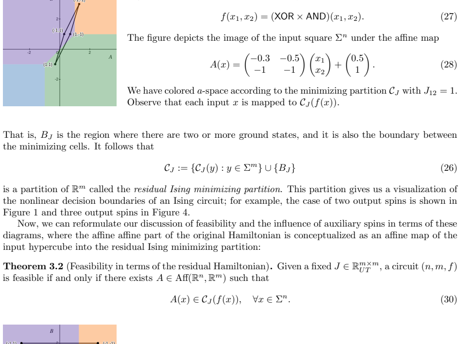
- Output-output couplings do real work: with one output bit the feasible circuits are exactly threshold functions (linear classifiers), while multi-output circuits can realize nonlinear functions such as XOR paired with AND.
- The no-local-minima condition is enforced by adding one linear inequality per input-wrong-output pair, so a designer can require fast, annealing-free convergence and still use linear programming.
- Because auxiliary (hidden) spins can be treated as ordinary outputs, the same geometric feasibility and local-minima machinery applies to circuits with hidden units.
- Energy graphs containing a directed spanning tree rooted at the correct output are exactly the no-local-minima constraint sets, which suggests an iterative LP refinement that lowers the L1 norm of the Hamiltonian.
Reading between the lines
- One route the paper leaves implicit: train an affine 1-NN embedding of a Boolean function (a convex problem in centroid placement) and then read off an Ising Hamiltonian; this would give a practical synthesis loop rather than solving the exponentially large LP directly.
- The local-minima-free inequality is testable on small circuits: a random benchmark comparing single-temperature greedy descent with and without the extra constraints should show the no-local-minima Hamiltonians solving every input exactly, while ordinary feasible Hamiltonians fail on a nonzero fraction.
- The injectivity requirement in Lemma 4.8 is the hinge: if some Voronoi-feasible circuit only admits degenerate (non-injective) solutions, Theorem 4.9's explicit Hamiltonian construction would need modification, though feasibility itself would not change.
- The tropical-geometry remark in Appendix D connects degeneracy loci to tropical hypersurfaces; a natural extension is to use tropical dimension counts to predict how many extra constraints the no-local-minima LP typically needs.
Editorial analysis
A structured set of objections, weighed in public.
Referee Report
Summary. This paper develops a geometric framework for zero-temperature Ising circuits. It introduces residual Hamiltonian diagrams, proves that feasibility of a circuit is equivalent to the existence of an affine map sending each input into the appropriate minimizing cell (Theorem 3.2), and then presents two main structural results: Theorem 4.9, which claims that every affine 1-NN-feasible circuit whose centroids are an affine image of the hypercube is feasible as an Ising circuit, and Theorem 5.8 with Corollary 5.9, which give a linear sufficient condition for the energy landscape to have no local minima other than the desired output. The paper also contains empirical classifications of small circuits and a short tropical-geometry appendix.
Significance. If the results stand, the paper provides a genuinely useful design principle: the decision structure of affine 1-NN classifiers can be realized by low-temperature Ising Hamiltonians, and the elimination of parasitic local minima reduces to adding linear inequalities to the inverse-Ising linear program. The central theorems are derived from definitions rather than fitted parameters, and the proofs of Lemma 5.6, Theorem 5.8, and Theorem 3.2 are clean and self-contained. The no-local-minima result in particular is constructive and immediately usable for small circuits. The main caveat is that the proof of Theorem 4.9 currently has a genuine gap in the use of Lemma 4.7; the gap is localized and appears repairable, so the paper merits revision rather than rejection.
major comments (2)
- [Section 4, Lemma 4.7 and Theorem 4.9 (Eqs. (53), (67)-(70))] The proof of Theorem 4.9 uses Lemma 4.7 in the form -B^*(V_{B(Σ^m)}(By)) = C_{J_T}(y), which requires B to be injective as an affine map R^m → R^n, i.e. T must have full column rank. Lemma 4.8, as stated and sketched, guarantees only that B is injective on the finite set Σ^m. These hypotheses are not equivalent: for example, with m = n = 2, take T = u a^T with u = (1,1.5) and a = (1,π); the affine map B(y) = T y + b is injective on Σ^2 because no difference of two hypercube points is annihilated by a^T, yet T has rank one, so -B^* maps R^2 onto a one-dimensional subspace while C_{J_T}(y) is open in R^2, making the equality in (53) false. The chain (67)-(70) therefore has a false intermediate step for exactly the Voronoi solutions that Lemma 4.8 supplies. The central claim appears salvageable, because the pointwise identity (55) does not require injectivity and yields the forward inclusion -B^*(V_{B(Σ^m)}(By)) ⊆ C_{J_T}(y), which suffices together with Theorem 3.2; but the manuscript must either prove a full-rank version of Lemma 4.8 or replace Lemma 4.7 by an inclusion argument.
- [Section 4, Lemma 4.8] The proof of Lemma 4.8 is only a sketch, with the details left to the reader, and the lemma is load-bearing for Theorem 4.9. A complete proof is needed. If the lemma is strengthened to produce a full-column-rank solution, the perturbation argument must avoid the finitely many rank-degeneracy hyperplanes in coefficient space while preserving the strict inequalities defining the Voronoi cells; if the weaker finite-injectivity version is kept, Theorem 4.9 must instead be proved by the inclusion argument described above. As written, the text does not allow the reader to verify either route.
minor comments (6)
- [Section 5, Definition 5.4] The energy graph definition contains a typo: the edge condition should be H(x,z) > H(x,y), not H(x,z) > H(y,z).
- [Section 5.1, Figure 9 caption] The caption says the red region has a global minimum of (1,-1) and a local minimum of (1,-1); the second state should presumably be (-1,1), matching the surrounding text.
- [Section 2.1.2, Lemma 2.6] The proof asserts that ϵ < δ, but only ϵ ≤ δ is guaranteed; the perturbation argument still works with a margin argument, so the inequality should be corrected or justified.
- [Appendix C, Proposition C.7] The exhaustive counts for shape (3,2) circuits are asserted without code, data, or a reproducibility protocol; if these empirical claims are retained, they should be backed by an available artifact or by a complete symbolic enumeration.
- [Appendix D] Appendix D ends mid-sentence with 'Similarly, it'; the passage should be completed or removed, and the notation ϵ_n versus ε_n should be made consistent.
- [Section 5.1.1] The iterative spanning-tree procedure is presented as an algorithm improvement but has no convergence guarantee or complexity analysis; it should be labeled as a heuristic unless those properties are supplied.
Circularity Check
No significant circularity: the main theorems are derived in-paper from explicit definitions; the only self-citations are peripheral and non-load-bearing.
full rationale
The paper's two central results are self-contained derivations. Theorem 4.9 (Ising circuits superset affine 1-NN classifiers) starts from Definition 4.5 of Voronoi feasibility and proves via Lemma 4.7's algebraic identity that a Voronoi solution B produces an explicit Ising Hamiltonian H(x,y) = -B*(x)·y + <J_T,y^⊗2>_F encoding f; the direction of implication (Voronoi feasible -> Ising feasible) is not assumed in the definition of feasibility. Theorem 5.8 and Corollary 5.9 derive the no-local-minima LP constraint directly from Lemma 5.6's characterization of local minima and from the algebra of EJ(a,z)-EJ(a,y); no fitted quantity is renamed as a prediction, and no external uniqueness theorem is imported. The only self-citations to the authors' prior work [7] (Section 2.2's pointer for the standard fact that auxiliary spins always make a circuit feasible via quadratization, and Appendix C.1's classification fact that an AND component renders XOR feasible) are peripheral to the main proofs; the central claims do not reduce to these citations. A separate rigor concern, not circularity: Lemma 4.8 proves injectivity only on the finite set Σ^m, while Lemma 4.7's proof uses B as an injective affine map, so the equality -B*(V_{B(Σ^m)}(By)) = C_{J_T}(y) is not justified for rank-deficient Voronoi solutions. This is a proof gap that can be repaired by an inclusion argument, not a circularity of the claimed derivation.
Assumptions & free parameters
assumptions (4)
- domain assumption Input spins can be pinned, so input biases and input-input couplings can be set to zero.
- domain assumption Computation is defined in the zero-temperature limit with a unique ground state.
- domain assumption Every Boolean function is feasible given enough auxiliary spins (polynomial quadratization).
- standard math Standard convex-geometry and threshold-function facts.
Cite this review
Pith. "Pith review of Geometric Theory of Ising Machines." pith.science (2026). https://pith.science/paper/WDIOXABS
@misc{pith2026250712626,
  author       = {Pith},
  title        = {Pith review of: Geometric Theory of Ising Machines},
  year         = {2026},
  howpublished = {\url{https://pith.science/paper/WDIOXABS}},
  note         = {Machine review of arXiv:2507.12626}
}
read the original abstract
We contribute to the mathematical theory of the design of low temperature Ising machines, a type of experimental probabilistic computing device implementing the Ising model. Encoding the output of a function in the ground state of a physical system allows efficient and distributed computation, but the design of the energy function is a difficult puzzle. We introduce a diagrammatic device that allows us to visualize the decision boundaries for Ising circuits. It is then used to prove two results: (1) Ising circuits are a generalization of 1-NN classifiers with a certain special structure, and (2) Elimination of local minima in the energy landscape can be formulated as a linear programming problem.
Figures


Figures from the paper (8 more)


Reference graph
Works this paper leans on
-
[1]
Endre Boros and Peter L. Hammer. “Pseudo-Boolean optimization”. In: Discrete Applied Mathematics 123.1 (2002), pp. 155–225. issn: 0166-218X. doi: 10.1016/S0166-218X(01)00341-9
-
[2]
Analog Coupled Oscillator Based Weighted Ising Machine
Jeffrey Chou, Suraj Bramhavar, et al. Analog Coupled Oscillator Based Weighted Ising Machine . 2019. arXiv: 1906.06312 [physics.comp-ph]
work page Pith review arXiv 2019
-
[3]
Linear Separability Of The Vertices Of An n-Dimensional Hypercube
Nicolle Gruzling. Linear Separability Of The Vertices Of An n-Dimensional Hypercube . 2007. doi: 10.24124
work page 2007
-
[4]
Sze-Tsen Hu. Threshold logic. University of California Press, Berkeley and Los Angeles, 1965
work page 1965
-
[5]
Solving Boltzmann Optimization Problems with Deep Learning
Fiona Knoll, John T. Daly, and Jess J. Meyer. Solving Boltzmann Optimization Problems with Deep Learning. 2024. arXiv: 2401.17408 [cs.LG]. url: https://arxiv.org/abs/2401.17408
work page Pith review arXiv 2024
-
[6]
Ising formulations of many NP problems
Andrew Lucas. “Ising formulations of many NP problems”. In: Frontiers in Physics 2 (2014). issn: 2296-424X. doi: 10.3389/fphy.2014.00005
arXiv 2014
-
[7]
Design of General Purpose Minimal-Auxiliary Ising Ma- chines
Isaac K. Martin, Andrew G. Moore, et al. “Design of General Purpose Minimal-Auxiliary Ising Ma- chines”. In: 2023 IEEE International Conference on Rebooting Computing (ICRC) . 2023, pp. 1–10. doi: 10.1109/ICRC60800.2023.10386525
-
[8]
A fully programmable 100-spin coherent Ising machine with all-to-all connections
Peter L. McMahon, Alireza Marandi, et al. “A fully programmable 100-spin coherent Ising machine with all-to-all connections”. In:Science 354.6312 (2016), pp. 614–617.doi: 10.1126/science.aah5178
Show all 16 references
-
[9]
Thermodynamic computing system for AI applica- tions
Denis Melanson, Mohammad Abu Khater, et al. “Thermodynamic computing system for AI applica- tions”. In: Nature Communications 16.1 (2025), p. 3757. doi: 10.1038/s41467-025-59011-x
2025 doi
-
[10]
McMahon, and Tim Byrnes
Naeimeh Mohseni, Peter L. McMahon, and Tim Byrnes. Ising machines as hardware solvers of com- binatorial optimization problems . 2022. arXiv: 2204.00276 [quant-ph]. url: https://arxiv.org/ abs/2204.00276
2022 arXiv
-
[11]
Inverse statistical problems: from the inverse Ising problem to data science
H. Chau Nguyen, Riccardo Zecchina, and Johannes Berg. “Inverse statistical problems: from the inverse Ising problem to data science”. In: Advances in Physics 66.3 (June 2017), pp. 197–261. issn: 1460-
2017
-
[12]
Experiments with an oscillator based Ising machine
Shrish Roy and Bernd Ulmann. Experiments with an oscillator based Ising machine . 2025. arXiv: 2502.03167 [cs.ET]. url: https://arxiv.org/abs/2502.03167
2025 arXiv
-
[13]
Designing Unit Ising Models for Logic Gate Simulation through Integer Linear Programming
Shunsuke Tsukiyama, Koji Nakano, et al. Designing Unit Ising Models for Logic Gate Simulation through Integer Linear Programming. 2024. arXiv: 2406.18130 [cs.ET]. url: https://arxiv.org/ abs/2406.18130
2024 arXiv
-
[14]
Coherent Ising machines—optical neural networks operating at the quantum limit
Yoshihisa Yamamoto, Kazuyuki Aihara, et al. “Coherent Ising machines—optical neural networks operating at the quantum limit”. In: npj Quantum Information 3.1 (2017), p. 49. doi: 10 . 1038 / s41534-017-0048-9
2017
-
[15]
250 Magnetic Tunnel Junctions-Based Probabilistic Ising Ma- chine
Shuhan Yang, Andrea Grimaldi, et al. 250 Magnetic Tunnel Junctions-Based Probabilistic Ising Ma- chine. 2025. arXiv: 2506.14590 [cond-mat.mtrl-sci]. url: https://arxiv.org/abs/2506.14590. 26
2025 arXiv
-
[6976]
url: http://dx.doi.org/10.1080/00018732.2017
doi: 10.1080/00018732.2017.1341604 . url: http://dx.doi.org/10.1080/00018732.2017. 1341604. 25
2017
Reviewed August 6, 2026 · model on record in the stance chip above.
Discussion (0). Continue with ORCID to comment.