Detailed study of ELAIS N1 field with the uGMRT -- II. Source Properties and Spectral Variation Of Foreground Power Spectrum from 300-500 MHz Observations

Abhirup Datta; Arnab Chakraborty; Huib Intema; Kanan K. Datta; Madhurima Choudhury; Nirupam Roy; Prasun Dutta; Samir Choudhuri; Somnath Bharadwaj; Srijita Pal

REVIEW 3 major objections 5 minor 2 cited by

Detailed study of ELAIS N1 field with the uGMRT -- II. Source Properties and Spectral Variation Of Foreground Power Spectrum from 300-500 MHz Observations

T0 review · 3 major / 5 minor · reviewed 2026-08-14 · deepseek-v4-flash

Challenge this review Re-run · record.json Download PDF Read on arXiv ↗ Review JSON

Pith's one-line read Using 300-500 MHz uGMRT observations of ELAIS N1, this paper measures the frequency scaling of the diffuse Galactic synchrotron foreground power spectrum and finds a spectral index α = 2.9 ± 0.21 at multipole 1200.

desk verdict Genuinely new wide-band interferometric MFAPS measurement of Galactic synchrotron spectral variation, carefully made and honestly hedged; the main assumption to probe is that residual point sources do not bias the fitted alpha. read the letter →

arxiv 1908.10380 v2 pith:WGKKMNAG submitted 2019-08-27 astro-ph.CO

Arnab Chakraborty , Nirupam Roy , Abhirup Datta , Samir Choudhuri , Kanan K. Datta , Prasun Dutta , Somnath Bharadwaj , Huib Intema

show 3 more authors

Madhurima Choudhury Srijita Pal Tirthankar Roy Choudhury

This is my paper · ORCID

classification astro-ph.CO

keywords radiocontinuum:galaxiesdiffuseGalacticsynchrotronemissionangularpowerspectrumforegroundsEpochofReionization21cmcosmologysourcecountsuGMRTobservations

verification ladder T0 review T1 audit T2 compute T3 formal

The pith

A machine-rendered reading of the paper's core claim, the machinery that carries it, and where it could break.

The reading

This paper uses 25 hours of upgraded Giant Metrewave Radio Telescope (uGMRT) observations of the ELAIS N1 field across 300-500 MHz to build a 2528-source catalog and, for the first time, measure how the angular power spectrum of diffuse Galactic synchrotron emission (DGSE) changes with frequency over that band. The key result is the Multi-Frequency Angular Power Spectrum (MFAPS): the amplitude at angular multipole $\ell_0 = 1200$ follows $C_\ell(\nu) = A \nu^{-2\alpha}$ with $\alpha = 2.9 \pm 0.21$. Because the DGSE foreground is orders of magnitude brighter than the redshifted 21 cm signal, knowing whether it is spectrally smooth enough to subtract is a central input for Epoch of Reionization experiments. A single power law and a broken power law (break at 405 MHz) both fit the data, so the paper establishes the measurement without finally deciding which model is correct.

What carries the argument

The central mechanism is the subtraction-and-estimation chain. UVSUB removes the CLEAN point-source model from the calibrated visibilities, leaving a residual dominated by DGSE plus faint residual sources. The Tapered Gridded Estimator (TGE), a visibility-correlation estimator that grids the visibilities and removes the noise-bias term by excluding self-correlation, then provides unbiased estimates of the angular power spectrum $C_\ell$ for each 8 MHz sub-band. A tapering parameter of $f = 0.5$ confines the effective field of view so the estimated $C_\ell$ is not affected by direction-dependent calibration effects, as established in the companion paper. The frequency evolution is tested by normalizing each sub-band spectrum at $\ell_0 = 1200$ and fitting $C_{\ell_0}(\nu) = A \nu^{-2\alpha}$, with an alternative broken power-law model; the angular power-law index $\beta$ across sub-bands lies between about 1.8 and 3.

What would settle it

Run the same MFAPS analysis after injecting and subtracting a simulated population of faint point sources just below the 100 $\mu$Jy catalog limit; if the fitted $C_{\ell_0=1200}(\nu)$ amplitudes change by more than the quoted errors, especially toward higher frequencies where faint source counts are largest, then the measured $\alpha = 2.9 \pm 0.21$ is contaminated by unresolved sources rather than being the true DGSE spectral index.

Watch

Extended reading notes

Core claim

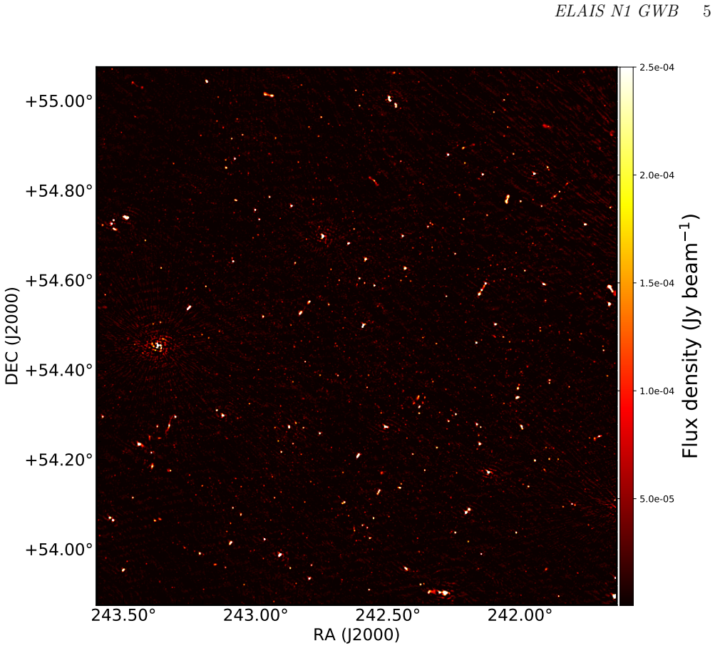
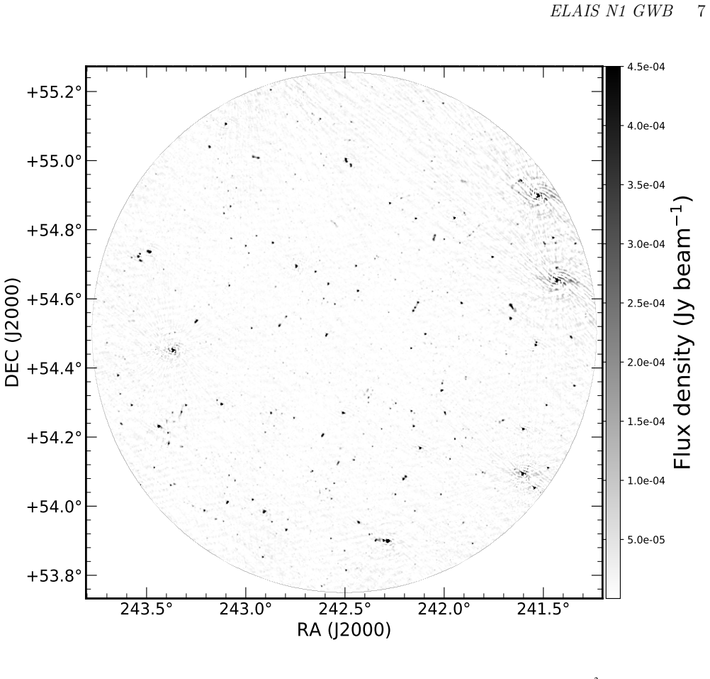
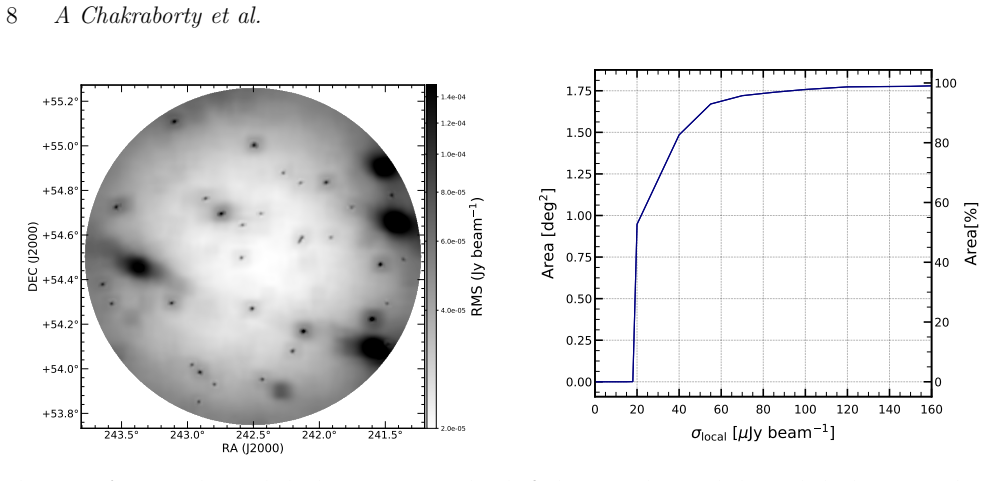
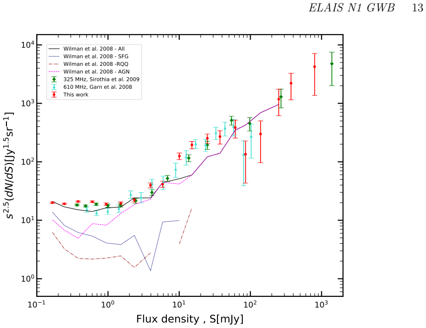
The paper's central claim has two parts. First, a deep 400 MHz image with rms noise of about 15 $\mu$Jy beam$^{-1}$ over roughly 1.8 deg$^2$ yields a catalog of 2528 sources above 100 $\mu$Jy; the normalized Euclidean source counts are consistent with earlier 325 MHz and 610 MHz observations of the same field and with the SKADS simulation, and the flattening below about 1 mJy is attributed to a rising population of star-forming galaxies and radio-quiet AGN. Second, and more central to the paper's novelty, is the spectral characterization of foreground fluctuations: after subtracting the CLEAN point-source model from the calibrated visibilities, the residual emission is treated as DGSE and analyzed with the Tapered Gridded Estimator in 8 MHz chunks, of which 13 are usable. The angular power spectrum amplitude at $\ell_0 = 1200$ is fitted as $C_\ell(\nu) = A \nu^{-2\alpha}$ over 300-500 MHz, giving $\alpha = 2.9 \pm 0.21$ with reduced chi-square 1.6. A broken power law with a break at 405 MHz, $\alpha_1 = 2.1 \pm 0.2$ and $\alpha_2 = 4.8 \pm 0.4$, gives reduced chi-square 0.3, but the paper states explicitly that the error bars do not allow either model to be ruled out, so a single spectral index remains viable.

Load-bearing premise

The result depends on the assumption that the emission left over after modelling and subtracting individual radio sources is truly the diffuse synchrotron glow of the Galaxy, and that the estimator recovers its power spectrum without being skewed by calibration or ionospheric errors; if faint unresolved sources contribute differently at different frequencies, the fitted spectral index would be biased.

Editorial extensions

If this is right

If the single power law holds, foreground models for 21 cm experiments can use a spectral index near 2.9 for this field, providing a direct empirical scaling $C_\ell(\nu) \propto \nu^{-2\alpha}$ for foreground subtraction.
If the broken power law is real, the steepening above 405 MHz implies that the diffuse foreground is not perfectly spectrally smooth, and foreground-removal schemes that assume a constant spectral index would leave frequency-dependent residuals in the EoR window.
The source catalog and normalized source counts supply a point-source foreground model down to 100 $\mu$Jy for the ELAIS N1 field, which can be subtracted before diffuse foreground analysis in future 21 cm observations.
Because the measured MFAPS is consistent with previous total-power spectral index measurements, the result strengthens the empirical basis for treating DGSE as spectrally smooth while quantifying how much spectral structure remains.
The data also show that wide-band interferometric observations can probe foreground spectral structure directly, rather than relying only on two-frequency comparisons.

Reading between the lines

Editorial extensions of the paper, not claims the author makes directly.

The same residual-visibility method could be applied to other high-latitude fields to test whether the MFAPS spectral index is universal or varies with sky position; if it varies, foreground subtraction codes will need spatially varying spectral models.
A deeper or wider-band observation that resolves and subtracts the residual point-source population below 100 $\mu$Jy would directly separate unresolved-source contamination from true DGSE spectral structure and could decide between the single and broken power laws.
If the spectral break near 405 MHz is confirmed, the steepening tied to synchrotron aging would constrain the electron population responsible for small-scale fluctuations in this field, giving a testable link to cosmic-ray electron models.
The TGE-on-residual approach could provide measurement-driven foreground spectral priors for 21 cm intensity mapping, reducing reliance on all-sky total-power maps at lower resolution.

Share X Bluesky LinkedIn Reddit HN

Signed reviews

No signed human review yet.

Editorial analysis

A structured set of objections, weighed in public.

Desk editor's note, referee report, and a circularity audit.

Desk Editor's Note

read the letter

Two things to know. First, the genuinely new result is in Section 7: a wide-band (300-500 MHz) interferometric estimate of the frequency dependence of the diffuse Galactic synchrotron angular power spectrum (MFAPS) in the ELAIS N1 field. Earlier work used two discrete frequencies or total-power measurements; this uses the full 200 MHz band. Second, the paper is properly cautious: it states plainly that a single power law (alpha = 2.9 +/- 0.21) cannot be ruled out against a broken power law, so the headline is a defensible first estimate, not an overclaim.

The source catalog and source counts are solid but confirmatory. The 2528-source catalog (100 uJy threshold) agrees with earlier GMRT 325/610 MHz catalogs of the field, flux scale is checked against NVSS, FIRST, and Garn et al. with median ratios near unity, astrometric offsets are around 0.5 arcsec, and the normalized counts match SKADS including the sub-mJy flattening. The FDR and completeness corrections rest on 100 injection simulations. That part is careful and believable, though the full catalog is not released and the primary-beam error test is described qualitatively rather than shown.

The soft spot is the foundation of the MFAPS estimate. The residual visibilities after UVSUB subtraction of the CLEAN model are assumed to be dominated by DGSE, with residual sources 'below the noise.' An undetected source population can still bias a power spectrum, and if that floor scales differently with frequency (a -0.7 source spectral index gives roughly nu^-1.4, much flatter than the claimed nu^-5.8 for DGSE), it will flatten the fitted frequency slope. The tapering f=0.5 meant to suppress direction-dependent calibration effects was validated in the companion paper at one 32 MHz band around 325 MHz, not across 300-500 MHz; that is a dependency on prior work, not a flaw by itself, but it is untested here. The data-dependent selection of the 'steep power law' l-range in each sub-band adds further room for the quoted alpha to move. The reduced chi^2 of 1.6 for the single power law and 0.3 for the hand-placed break at 405 MHz show unmodeled structure, and the paper acknowledges this. The measured alpha is consistent with EDGES (2.5-2.6) and La Porta (2.9-3.2) total-power values, which limits the damage. The stress-test concern that the break could be a contamination artifact is possible, but the paper never claims the break is real, so the risk to the actual conclusions is contained.

Who this is for: anyone modeling foregrounds for LOFAR, HERA, SKA-low, or uGMRT EoR programs. It deserves a serious referee. I would send it to review with a request that the authors quantify the residual-source floor, for example by injecting simulated point sources into the visibilities and checking how much the fitted alpha moves; releasing the catalog would also help. As it stands the measurement is a reasonable first constraint, not a benchmark to adopt blindly.

Referee Report

3 major / 5 minor

Summary. The paper presents a 300-500 MHz uGMRT observation of the ELAIS N1 field, yielding a 1.8 deg^2 image with ~15 uJy beam^-1 rms noise, a catalog of 2528 sources, comparisons with earlier radio catalogs, corrected Euclidean-normalized source counts, and a multi-frequency angular power spectrum (MFAPS) of diffuse Galactic synchrotron emission (DGSE). The central MFAPS result is a fit of C_l0(nu) = A nu^{-2 alpha} at l0=1200 over 13 sub-bands, giving alpha = 2.9 +/- 0.21 with reduced chi^2 = 1.6, together with a broken power-law fit (break at 405 MHz, alpha1 = 2.1 +/- 0.2, alpha2 = 4.8 +/- 0.4, reduced chi^2 = 0.3) that the authors explicitly state cannot be preferred over the single power law. The source counts flatten below ~1 mJy and agree with SKADS simulations and previous observations of the same field.

Significance. If the MFAPS estimate is unbiased, it is a genuinely useful new interferometric constraint on the spectral smoothness of low-frequency Galactic foregrounds in the 300-500 MHz band, a quantity directly relevant to 21-cm EoR experiments. The paper is careful in its flagging, calibration, source-count correction procedures, and error reporting; the source catalog and corrected counts are valuable products in their own right. The central alpha = 2.9 +/- 0.21 is a falsifiable prediction that can be checked by future wide-band measurements. The main caveats are that the MFAPS result rests on unquantified residual point-source power and on an assumed insensitivity to direction-dependent calibration that was previously validated only at a single band.

major comments (3)

[Sec. 7, Eq. (9)] The fitted spectral index alpha = 2.9 +/- 0.21 is derived from TGE amplitudes after UVSUB subtraction of the CLEAN point-source model, but the residual compact-source contribution to C_l is never estimated. The text says the residual data 'mainly consists of DGSE and residual point sources below the noise level,' and the l-range for each sub-band is chosen where a steep power law is seen; this does not exclude a frequency-dependent Poisson floor. Since the matched sources in Sec. 5.3 have median spectral index ~ -0.7, a residual source population contributes a component scaling roughly as nu^{-1.4}, much flatter than the DGSE scaling nu^{-2 alpha}; such a floor would bias the fitted alpha and could contribute to the apparent steepening above 405 MHz. I request a quantitative estimate of the residual point-source power, for example by injecting simulated sources below the detection threshold and propagating them through the same UVSUB+TGE pipeline, or by including a free residual-source term in the MFAPS fit.
[Sec. 7, Fig. 13] The l-range over which each sub-band is fit is chosen separately for each sub-band ('we have found a l range where C_l^i shows a steep power law behavior'), and the fitted beta_i values scatter between 1.8 and 3.0. The amplitude at l0 = 1200 is therefore not measured directly but obtained from a model-dependent fit whose range changes from band to band; this can introduce band-to-band systematic scatter in A_i that propagates into the quoted alpha. Please demonstrate robustness by repeating the MFAPS fit with a fixed l-range or a common selection rule across all sub-bands, and by reporting the sensitivity of alpha to the choice of l0.
[Sec. 7, tapering f = 0.5] The claim that tapering f = 0.5 makes the C_l estimates insensitive to direction-dependent calibration errors is imported from Chakraborty et al. (2019), where it was validated at a single 32-MHz band around 325 MHz. The present analysis uses 8-MHz sub-bands spanning 300-500 MHz, and ionospheric and calibration phase errors have different frequency dependence; no test is shown that the f = 0.5 choice remains unbiased across the full band. I ask for a direct check, for example by comparing the recovered MFAPS for two or more tapering parameters, or by comparing with an independently calibrated or direction-dependent-calibrated reduction.

minor comments (5)

[Abstract / Introduction] The phrase 'for the first time' should be qualified as the first wide-band interferometric estimate, since total-power measurements of the spectral index of diffuse emission already exist; this would avoid overclaiming novelty.
[Sec. 7, Eq. (9)] The statement that the reduced chi^2 of 1.6 is 'high' is not quite accurate for 11 degrees of freedom; please report chi^2, the number of degrees of freedom, and the resulting p-value so the reader can judge the fit quality.
[Fig. 14] The legend entry 'Arnab et al. 2019' should read 'Chakraborty et al. 2019' to match the reference list.
[Table 4] There is a typographical spacing error in the first flux-density bin of the sixth row: '1.218-1 935' should be '1.218-1.935'.
[Sec. 4] The text refers to 'PYBDM output' in the discussion of PSF variation; this appears to be a typo for 'PYBDSF output'.

Circularity Check

0 steps flagged · score 0.0 of 10

No significant circularity: the MFAPS spectral index is measured from independently estimated per-sub-band power spectra, not derived from its own inputs.

full rationale

The central MFAPS result (Eq. 9: C_l=1200(nu)=A nu^{-2 alpha}) is obtained by (i) subtracting the CLEAN point-source model with UVSUB, (ii) estimating C_l separately in 13 independent 8-MHz sub-bands with TGE, (iii) fitting each sub-band's angular spectrum over an l-range chosen for that sub-band, and (iv) fitting the frequency dependence of the resulting amplitudes. No parameter in the fit is defined in terms of the target spectral index, and the spectral index alpha=2.9±0.21 is not a renamed input: it is a free parameter fitted to 13 measured amplitudes. The 325 MHz point from Chakraborty et al. (2019) is used only as a consistency overlay, and the result is additionally benchmarked against external measurements (La Porta et al. 2008; Rogers & Bowman 2008; Mozdzen et al. 2017, 2019). The self-citation to Chakraborty et al. (2019) for the TGE tapering parameter f=0.5 is a methodological choice for the estimator; it affects the uncertainty budget but does not by construction determine the fitted alpha, so it is not load-bearing circularity. The data-dependent choice of l-range and the residual-point-source contamination are correctness risks, not circular steps: they could bias alpha but do not make the derivation equivalent to its inputs.

Assumptions & free parameters 7 free parameters · 6 assumptions · 0 invented entities

The central MFAPS measurement rests on the assumed C_l(ν) ∝ ν^{-2α} foreground model and on the assumption that point-source-subtracted visibilities trace only diffuse synchrotron emission. The tapering choice f=0.5 is inherited from a self-cited paper. The paper introduces no new physical entities; all parameters are either fitted amplitudes or slopes or chosen processing values, and the break frequency 405 MHz is fixed by hand. No code or data products are released.

free parameters (7)

Single power-law spectral index alpha = 2.9 ± 0.21
Fitted to 13 measured MFAPS amplitudes at l0=1200; central result of Sec. 7.
Amplitude A of single power law = not quoted in text (Fig. 14)
Normalization in C_l(ν)=A ν^{-2α}; fitted together with alpha.
Broken power-law alpha1 = 2.1 ± 0.2
Fitted below the fixed 405 MHz break in Eq. 10.
Broken power-law alpha2 = 4.8 ± 0.4
Fitted above the fixed break; the spectral steepening interpretation relies on this value.
Break frequency nu_break = 405 MHz
Fixed by hand in Eq. 10 rather than determined by the fit; not ruled out by the chi-square comparison.
Per-sub-band angular index beta_i = 1.8 to 3.1 (Fig. 13)
Power-law slopes fit to each of 13 sub-band APS; normalization at l0=1200 defines the MFAPS points.
Tapering fraction f = 0.5
Chosen in Sec. 7 based on Chakraborty et al. 2019 to suppress direction-dependent calibration effects; affects the estimated C_l.

assumptions (6)

domain assumption DGSE angular power spectrum follows C_l(ν) = A (l/l0)^{-β} (ν/ν0)^{-2α}
Adopted from Santos et al. 2005 and Datta et al. 2007 in Eq. 1 to interpret the measured power spectra.
domain assumption UVSUB removes all discrete sources; residual visibilities mainly contain DGSE plus sub-noise point sources
Sec. 7 states this; if incorrect, the measured C_l and alpha are biased by residual source power.
domain assumption TGE with tapering f=0.5 is unbiased without direction-dependent calibration
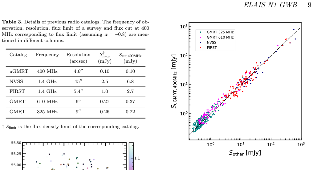
Asserted in Sec. 7 with reference to Chakraborty et al. 2019; not directly demonstrated for this data set.
domain assumption External catalogs and source counts are scaled to 400 MHz with a single spectral index alpha = -0.8
Used in Secs. 5 and 6.3; a distribution of intrinsic spectral indices would change the comparison.
domain assumption Completeness simulations assume dN/dS proportional to S^{-1.6} and 10% extended sources
Sec. 6.2 injects sources with this slope; the completeness correction depends on the assumed intrinsic counts.
domain assumption Synchrotron age interpretation assumes average magnetic field B = 10 microG
Sec. 7 derives 80 Myr from Eq. 1 of Carilli et al. 1991 using B=10 microG; the age and even the break depend on this assumption.

how reviews work

0 comments

Cite this review

Pith. "Pith review of Detailed study of ELAIS N1 field with the uGMRT -- II. Source Properties and Spectral Variation Of Foreground Power Spectrum from 300-500 MHz Observations." pith.science (2026). https://pith.science/paper/WGKKMNAG

@misc{pith2026190810380,
  author       = {Pith},
  title        = {Pith review of: Detailed study of ELAIS N1 field with the uGMRT -- II. Source Properties and Spectral Variation Of Foreground Power Spectrum from 300-500 MHz Observations},
  year         = {2026},
  howpublished = {\url{https://pith.science/paper/WGKKMNAG}},
  note         = {Machine review of arXiv:1908.10380}
}

abstract

Understanding the low-frequency radio sky in depth is necessary to subtract foregrounds in order to detect the redshifted 21 cm signal of neutral hydrogen from the Cosmic Dawn, Epoch of Reionization (EoR) and post-reionization era. In this second paper of the series, we present the upgraded Giant Metrewave Radio Telescope (uGMRT) observation of the ELAIS N1 field made at 300-500 MHz. The image covers an area of $\sim 1.8$ $\mathrm{deg}^{2}$ and has a central background rms noise of $\sim$ 15 $\mu \mathrm{Jy}$ $\mathrm{beam}^{-1}$. We present a radio source catalog containing 2528 sources (with flux densities > 100 $\mu$Jy) and normalized source counts derived from that. The detailed comparison of detected sources with previous radio observations is shown. We discuss flux scale accuracy, positional offsets, spectral index distribution and correction factors in source counts. The normalized source counts are in agreement with previous observations of the same field, as well as model source counts from the Square Kilometre Array Design Study (SKADS) simulation. It shows a flattening below $\sim$1 mJy which corresponds to rise in population of star forming galaxies and radio-quiet AGN. For the first time, we estimated the spectral characteristics of the angular power spectrum or Multi-Frequency Angular Power Spectrum (MFAPS) of diffuse Galactic synchrotron emission (DGSE) over the wide frequency bandwidth of $300-500$~MHz from radio interferometric observations. This work demonstrates the improved capabilities of the uGMRT.

Figures

Figures reproduced from arXiv: 1908.10380 by the authors.

**Figure 1.** Left panel: The uv-coverage of ELAIS N1 field in kλ using the uGMRT for 300-500 MHz bandwidth. Only 6% of the total data points has been plotted. Large bandwidth and long observational time results in a densely filled uv-plane. Right panel: The relative baseline distribution as a function `, where ` = 2πU. U is the baseline length. This illustrates the sensitivity of uGMRT at different angular scale to estimate the … view at source ↗

**Figure 2.** The above uGMRT image is zoomed-in total intensity image of ELIAS N1 at 400MHz (bandwidth 200MHz). The Central off-source noise is ∼ 15 µJy beam−1 . The image covers a central area of ∼ 1.2 deg2 . This illustrates that a large number of weak sources are detected due to high signal-to-noise ratio achieved here. two more times. After this loop, we have done the final delay and bandpass calibration for the primary cali… view at source ↗

**Figure 3.** Primary beam corrected image of ELIAS N1 at 400MHz. The image extends over an area of ∼ 1.8 deg2 . The off source rms at the center is ∼ 15 µJy beam−1 and beam size is 4.6 00 × 4.3 00 [PITH_FULL_IMAGE:figures/full_fig_p007_3.png] view at source ↗

Figures from the paper (9 more)

**Figure 4.** Figure 4: Left image is showing the local rms noise measured in the final map. Local noise is high near the bright sources and at the edge of FoV. Right: Cumulative area of the final map with a rms noise level below the given value. 5 10 100 500 1000 Speak/ L 0.5 1.0 5.0 10.0 20…

**Figure 5.** Figure 5: The ratio of integrated to peak flux density Sint/Speak as a function of signal-to-noise ratio Speak/σL of sources. Extended sources are shown in red and point-like sources in green. (time resolution). We have theoretically estimated the combined effect of ban…

**Figure 7.** Figure 7: Comparison of total flux density of compact sources measured at 400 MHz using uGMRT with other radio catalogs at different frequencies 325 MHz GMRT (green), 610 MHz GMRT (magenta), NVSS (blue), FIRST (red). The black dashed line corresponds to SuGMRT/ Sother = 1. 16th …

**Figure 6.** Figure 6: Map of the ratios of integrated flux densities for high signal-to-noise, compact and isolated uGMRT 400 MHz sources with respect to GMRT 610 MHz sources. The colorscale is showing the flux density ratio. selected only high signal-to-noise Speak > 10σ sources in bo…

**Figure 8.** Figure 8: Comparison between flux densities measured at 400 MHz (uGMRT) and predicted flux densities using 325 MHz (Sirothia et al. 2009) and FIRST catalog. The mean value of the ratio, (Spredicted/SuGMRT), is 1.02 ± 017. to Perley & Butler (2013) to put them in the same flux sc…

**Figure 10.** Figure 10: The histogram of measured spectral indices of sources in this field after matching with different catalogs using a 5 00 match radius. The black dashed line corresponds to α = -0.7. The median spectral indices with errors from 16th and 84th percentile for different cat…

**Figure 12.** Figure 12: Euclidian-normalized differential source counts for the uGMRT 400 MHz observation of ELAIS N1 field. The red circles show the observed source counts after correction factors have been applied. For comparison, we also plot 325 MHz (green) (Sirothia et al. 2009), 610 MH…

**Figure 13.** Figure 13: The estimated angular power spectrum (C` ) with with 1 − σ error bar (green curve) as a function of angular multipole ` for 13 sub-bands. The vertical dashed lines (in maroon) shows ` range to fit a power law model and the black dashed line shows the best-fitting, CM …

**Figure 14.** Figure 14: Angular power spectrum of DGSE normalized at l = 1200 as a function of frequency. The magenta triangle is the measured power spectrum of DGSE at 325 MHz (Chakraborty, et al. 2019). The observed values are consistent with the previous measurement. range we fit a power …

Discussion (0). Continue with ORCID to comment.

Forward citations

Cited by 2 Pith papers

Reviewed papers in the Pith corpus that reference this work. Sorted by Pith novelty score. Full citation record

Intensity fluctuations of radio halo in galaxy cluster: Insights from power spectrum estimation
astro-ph.CO 2026-07 conditional novelty 6.0 of 10

Angular power spectra of 610 MHz radio halos show excess power-law fluctuations only in Abell 2744, requiring multiplicative C_ℓ ∝ ℓ^{-3} structure atop an exponential profile and consistent with ICM turbulence.
Investigating radio source population $\&$ spatial characteristics of diffuse Galactic synchrotron emission in the GAMA-23 field with uGMRT Band-3
astro-ph.GA 2026-08 conditional novelty 4.0 of 10

A 325 MHz uGMRT mosaic of the GAMA-23 field yields a 5741-source catalog, source counts, spectral indices, and angular power spectra of diffuse Galactic synchrotron emission.

Reference graph

Works this paper leans on

121 extracted references · 72 canonical work pages · cited by 2 Pith papers

[1]

D., Allende Prieto C., et al., 2015, ApJS, 219, 12

Alam S., Albareti F. D., Allende Prieto C., et al., 2015, ApJS, 219, 12

2015
[2]

S., Bharadwaj S., Chengalur J

Ali S. S., Bharadwaj S., Chengalur J. N., 2008, MNRAS, 385, 2166

2008
[3]

Barkana R., 2016, PhR, 645, 1

2016
[4]

A., Brown M

Battye R. A., Brown M. L., Browne I. W. A., et al., 2012, arXiv, arXiv:1209.1041

arXiv 2012
[5]

E., Amiri M., et al., 2014, SPIE, 9145, 914522

Bandura K., Addison G. E., Amiri M., et al., 2014, SPIE, 9145, 914522

2014
[6]

Baars J. W. M., Genzel R., Pauliny-Toth I. I. K., Witzel A., 1977, A&A, 61, 99

1977
[7]

H., White R

Becker R. H., White R. L., Helfand D. J., 1995, ApJ, 450, 559

1995
[8]

H., Fan X., White R

Becker R. H., Fan X., White R. L., et al., 2001, AJ, 122, 2850

2001

Show all 121 references

[9]

G., Brentjens M

Bernardi G., de Bruyn A. G., Brentjens M. A., et al., 2009, A&A, 500, 965

2009
[10]

Bernardi G., Zwart J. T. L., Price D., et al., 2016, MNRAS, 461, 2847

2016
[11]

K., 2001, JApA, 22, 293

Bharadwaj S., Sethi S. K., 2001, JApA, 22, 293

2001
[12]

B., Sethi S

Bharadwaj S., Nath B. B., Sethi S. K., 2001, JApA, 22, 21

2001
[13]

B., Sethi S

Bharadwaj S., Nath B. B., Sethi S. K., 2002, IAUS, 199, 108

2002
[14]

K., 2003, JApA, 24, 23

Bharadwaj S., Pandey S. K., 2003, JApA, 24, 23

2003
[15]

S., 2005, MNRAS, 356, 1519

Bharadwaj S., Ali S. S., 2005, MNRAS, 356, 1519

2005
[16]

D., Morales M

Bowman J. D., Morales M. F., Hewitt J. N., 2009, ApJ, 695, 183

2009
[17]

D., Rogers A

Bowman J. D., Rogers A. E. E., Monsalve R. A., Mozdzen T. J., Mahesh N., 2018, Natur, 555, 67

2018
[18]

J., 2015, aska.conf, Proc

Bull P., Camera S., Raccanelli A., Blake C., Ferreira P., Santos M., Schwarz D. J., 2015, aska.conf, Proc. Sci., Advancing Astrophysics with the Square Kilometre Array, PoS(AASKA14)24. (arXiv:1501.04088)

2015 arXiv
[19]

F., Hazelton B., et al., 2018, arXiv, arXiv:1811.01378

Byrne R., Morales M. F., Hazelton B., et al., 2018, arXiv, arXiv:1811.01378

2018 arXiv
[20]

O., Lazio J., Bale S., et al., 2012, AdSpR, 49, 433

Burns J. O., Lazio J., Bale S., et al., 2012, AdSpR, 49, 433

2012
[21]

D., Cairns I., Kaplan D

Bowman J. D., Cairns I., Kaplan D. L., et al., 2013, PASA, 30, e031

2013
[22]

L., Perley R

Carilli C. L., Perley R. A., Dreher J. W., Leahy J. P., 1991, ApJ, 383, 554

1991
[23]

Chakraborty A., et al., 2019, MNRAS, 487, 4102

2019
[24]

B., Harker G., et al., 2012, MNRAS, 423, 2518

Chapman E., Abdalla F. B., Harker G., et al., 2012, MNRAS, 423, 2518

2012
[25]

B., Bobin J., et al., 2013, MNRAS, 429, 165

Chapman E., Abdalla F. B., Bobin J., et al., 2013, MNRAS, 429, 165

2013
[26]

Sci., Advancing Astrophysics with the Square Kilometre Array, PoS(AASKA14)05

Chapman E., Bonaldi A., Harker G., et al., 2015,aska.conf, Proc. Sci., Advancing Astrophysics with the Square Kilometre Array, PoS(AASKA14)05. (arXiv:1501.04429)

2015 arXiv
[27]

B., Dulwich F., Jeli \'c V., Mort B., 2016, MNRAS, 458, 2928

Chapman E., Zaroubi S., Abdalla F. B., Dulwich F., Jeli \'c V., Mort B., 2016, MNRAS, 458, 2928

2016
[28]

P., Wang R

Chen Z. P., Wang R. L., Peterson J., Chen X. L., Zhang J. Y., Shi H. L., 2016, SPIE, 9906, 99065W

2016
[29]

S., 2014, MNRAS, 445, 4351

Choudhuri S., Bharadwaj S., Ghosh A., Ali S. S., 2014, MNRAS, 445, 4351

2014
[30]

S., Roy N., Ghosh A., 2016, MNRAS, 463, 4093

Choudhuri S., Bharadwaj S., Chatterjee S., Ali S. S., Roy N., Ghosh A., 2016, MNRAS, 463, 4093

2016
[31]

S., Roy N., Intema H

Choudhuri S., Bharadwaj S., Ali S. S., Roy N., Intema H. T., Ghosh A., 2017, MNRAS, 470, L11

2017
[32]

Ciliegi P., 1999, ASPC, 176, 355

1999
[33]

J., 1992, ARA&A, 30, 575

Condon J. J., 1992, ARA&A, 30, 575

1992
[34]

J., Cotton W

Condon J. J., Cotton W. D., Greisen E. W., Yin Q. F., Perley R. A., Taylor G. B., Broderick J. J., 1998, AJ, 115, 1693

1998
[35]

J., et al., 2012, ApJ, 758, 23

Condon J. J., et al., 2012, ApJ, 758, 23

2012
[36]

R., 2004, ApJ, 606, L5

Cooray A., Furlanetto S. R., 2004, ApJ, 606, L5

2004
[37]

L., 2009, ApJ, 703, 1851

Datta A., Bhatnagar S., Carilli C. L., 2009, ApJ, 703, 1851

2009
[38]

D., Carilli C

Datta A., Bowman J. D., Carilli C. L., 2010, ApJ, 724, 526

2010
[39]

K., Choudhury T

Datta K. K., Choudhury T. R., Bharadwaj S., 2007, MNRAS, 378, 119

2007
[40]

Dayal P., Ferrara A., 2018, PhR, 780, 1

2018
[41]

R., Parsons A

DeBoer D. R., Parsons A. R., Aguirre J. E., et al., 2017, PASP, 129, 045001

2017
[42]

M., Jonas J., Landecker T

de Oliveira-Costa A., Tegmark M., Gaensler B. M., Jonas J., Landecker T. L., Reich P., 2008, MNRAS, 388, 247

2008
[43]

J., 2002, ApJ, 564, 576

Di Matteo T., Perna R., Abel T., Rees M. J., 2002, ApJ, 564, 576

2002
[44]

Di Matteo T., Ciardi B., Miniati F., 2004, MNRAS, 355, 1053

2004
[45]

S., Tegmark M., Liu A., et al., 2015, PhRvD, 91, 023002

Dillon J. S., Tegmark M., Liu A., et al., 2015, PhRvD, 91, 023002

2015
[46]

B., 1958, PIRE, 46, 240

Field G. B., 1958, PIRE, 46, 240

1958
[47]

Franzen T. M. O., Banfield J. K., Hales C. A., et al., 2015, MNRAS, 453, 4020

2015
[48]

Franzen T. M. O., Vernstrom T., Jackson C. A., Hurley-Walker N., Ekers R. D., Heald G., Seymour N., White S. V., 2019, PASA, 36, e004

2019
[49]

R., Oh S

Furlanetto S. R., Oh S. P., Briggs F. H., 2006, PhR, 433, 181

2006
[50]

S., Chengalur J

Ghosh A., Bharadwaj S., Ali S. S., Chengalur J. N., 2011, MNRAS, 411, 2426

2011
[51]

S., Chengalur J

Ghosh A., Prasad J., Bharadwaj S., Ali S. S., Chengalur J. N., 2012, MNRAS, 426, 3295

2012
[52]

A., Riley J

Garn T., Green D. A., Riley J. M., Alexander P., 2008, MNRAS, 383, 75

2008
[53]

L., Williams W., Jarvis M

Hale C. L., Williams W., Jarvis M. J., et al., 2019, A&A, 622, A4

2019
[54]

Haslam C. G. T., Salter C. J., Stoffel H., Wilson W. E., 1982, A&AS, 47, 1

1982
[55]

R., Hancock P

Hurley-Walker N., Callingham J. R., Hancock P. J., et al., 2017, MNRAS, 464, 1146

2017
[56]

Iacobelli M., Haverkorn M., Orr \'u E., et al., 2013, A&A, 558, A72

2013
[57]

T., van Weeren R

Intema H. T., van Weeren R. J., R \"o ttgering H. J. A., Lal D. V., 2011, A&A, 535, A38

2011
[58]

T., Jagannathan P., Mooley K

Intema H. T., Jagannathan P., Mooley K. P., Frail D. A., 2017, A&A, 598, A78

2017
[59]

A., Wall J

Jackson C. A., Wall J. V., 1999, MNRAS, 304, 160

1999
[60]

G., Mevius M., et al., 2014, A&A, 568, A101

Jeli \'c V., de Bruyn A. G., Mevius M., et al., 2014, A&A, 568, A101

2014
[61]

Jeli \'c V., Zaroubi S., Labropoulos P., et al., 2008, MNRAS, 389, 1319

2008
[62]

G., Koopmans L

Jeli \'c V., Zaroubi S., Labropoulos P., Bernardi G., de Bruyn A. G., Koopmans L. V. E., 2010, MNRAS, 409, 164

2010
[63]

C., Trott C

Joseph R. C., Trott C. M., Wayth R. B., 2018, AJ, 156, 285

2018
[64]

Sci., Advancing Astrophysics with the Square Kilometre Array, PoS(AASKA14)01

Koopmans L., Pritchard J., Mellema G., et al., 2015, aska.conf, Proc. Sci., Advancing Astrophysics with the Square Kilometre Array, PoS(AASKA14)01. (arXiv:1505.07568 )

2015 arXiv
[65]

La Porta L., Burigana C., Reich W., Reich P., 2008, A&A, 479, 641

2008
[66]

C., Hazelton B

Li W., Pober J. C., Hazelton B. J., et al., 2018, ApJ, 863, 170

2018
[67]

Liu A., Tegmark M., 2011, PhRvD, 83, 103006

2011
[68]

R., 2013, fgu..book, ISBN: 9780691144917

Loeb A., Furlanetto S. R., 2013, fgu..book, ISBN: 9780691144917. Princeton, NJ: Princeton University Press

2013
[69]

Madau P., 1997, seim.proc, Proceedings of the 13th IAP Astrophysics Colloquium, Institut d'Astrophysique, Paris, France Publisher: Paris: Editions Frontieres, ISBN: 286332229X, 1997., p.295

1997
[70]

P., Waters B., Schiebel D., Young W., Golap K., 2007, ASPC..376, 127, ASPC..376

McMullin J. P., Waters B., Schiebel D., Young W., Golap K., 2007, ASPC..376, 127, ASPC..376

2007
[71]

Mohan N., Rafferty D., 2015, ascl.soft, ascl:1502.007

2015
[72]

K., 2018, MNRAS, 474, 1390

Mondal R., Bharadwaj S., Datta K. K., 2018, MNRAS, 474, 1390

2018
[73]

T., Datta K

Mondal R., Bharadwaj S., Iliev I. T., Datta K. K., Majumdar S., Shaw A. K., Sarkar A. K., 2019, MNRAS, 483, L109

2019
[74]

A., Rogers A

Monsalve R. A., Rogers A. E. E., Bowman J. D., Mozdzen T. J., 2017, ApJ, 835, 49

2017
[75]

F., Wyithe J

Morales M. F., Wyithe J. S. B., 2010, ARA&A, 48, 127

2010
[76]

J., Bowman J

Mozdzen T. J., Bowman J. D., Monsalve R. A., Rogers A. E. E., 2017, MNRAS, 464, 4995

2017
[77]

J., Mahesh N., Monsalve R

Mozdzen T. J., Mahesh N., Monsalve R. A., Rogers A. E. E., Bowman J. D., 2019, MNRAS, 483, 4411

2019
[78]

G., Trott C

Murray S. G., Trott C. M., Jordan C. H., 2017, ApJ, 845, 7

2017
[79]

T., Spangler S

Myers S. T., Spangler S. R., 1985, ApJ, 291, 52

1985
[80]

B., Bandura K., Bucher M

Newburgh L. B., Bandura K., Bucher M. A., et al., 2016, SPIE, 9906, 99065X

2016
[81]

R., Bradley R

Neben A. R., Bradley R. F., Hewitt J. N., et al., 2016, ApJ, 826, 199

2016
[82]

P., 2017, NatAs, 1, 671

Norris R. P., 2017, NatAs, 1, 671

2017
[83]

R., de Bruyn A

Offringa A. R., de Bruyn A. G., Biehl M., Zaroubi S., Bernardi G., Pandey V. N., 2010, MNRAS, 405, 155

2010
[84]

R., de Bruyn A

Offringa A. R., de Bruyn A. G., Zaroubi S., Biehl M., 2010, rfim.work, 36

2010
[85]

R., van de Gronde J

Offringa A. R., van de Gronde J. J., Roerdink J. B. T. M., 2012, A&A, 539, A95

2012
[86]

R., Pober J

Parsons A. R., Pober J. C., Aguirre J. E., Carilli C. L., Jacobs D. C., Moore D. F., 2012, ApJ, 756, 165

2012
[87]

R., Liu A., Aguirre J

Parsons A. R., Liu A., Aguirre J. E., et al., 2014, ApJ, 788, 106

2014
[88]

A., Butler B

Perley R. A., Butler B. J., 2013, ApJS, 204, 19

2013
[89]

C., Parsons A

Pober J. C., Parsons A. R., Aguirre J. E., et al., 2013, ApJ, 768, L36

2013
[90]

C., Parsons A

Pober J. C., Parsons A. R., DeBoer D. R., et al., 2013, AJ, 145, 65

2013
[91]

Prandoni I., 2018, IAUS, 333, 175

2018
[92]

Prandoni I., Guglielmino G., Morganti R., Vaccari M., Maini A., R \"o ttgering H. J. A., Jarvis M. J., Garrett M. A., 2018, MNRAS, 481, 4548

2018
[93]

R., Loeb A., 2012, RPPh, 75, 086901

Pritchard J. R., Loeb A., 2012, RPPh, 75, 086901

2012
[94]

J., 2011, A&A, 532, A71

Rau U., Cornwell T. J., 2011, A&A, 532, A71

2011
[95]

Reich P., Reich W., 1988, A&AS, 74, 7

1988
[96]

Rogers A. E. E., Bowman J. D., 2008, AJ, 136, 641

2008
[97]

G., Cooray A., Knox L., 2005, ApJ, 625, 575

Santos M. G., Cooray A., Knox L., 2005, ApJ, 625, 575

2005
[98]

Sci., Cosmology from a SKA HI intensity mapping survey

Santos M., Bull P., Alonso D., et al., 2015, Proc. Sci., Cosmology from a SKA HI intensity mapping survey. SISSA, Trieste, PoS(AASKA14)019. (arXiv:1501.03989)

2015 arXiv
[99]

A., Windhorst R

Shaver P. A., Windhorst R. A., Madau P., de Bruyn A. G., 1999, A&A, 345, 380

1999
[100]

Simpson C., 2017, RSOS, 4, 170522

2017
[101]

E., Wayth R

Sokolowski M., Tremblay S. E., Wayth R. B., et al., 2015, PASA, 32, e004

2015
[102]

K., Rao A

Swarup G., Ananthakrishnan S., Kapahi V. K., Rao A. P., Subrahmanya C. R., Kulkarni V. K., 1991, CuSc, 60, 95

1991
[103]

K., Dennefeld M., Saikia D

Sirothia S. K., Dennefeld M., Saikia D. J., Dole H., Ricquebourg F., Roland J., 2009, ASPC, 407, 27

2009
[104]

U., Rao M

Singh S., Subrahmanyan R., Shankar N. U., Rao M. S., Girish B. S., Raghunathan A., Somashekar R., Srivani K. S., 2018, ExA, 45, 269

2018
[105]

W., Tasse C., Hardcastle M

Shimwell T. W., Tasse C., Hardcastle M. J., et al., 2019, A&A, 622, A1

2019
[106]

R., Manoharan P

Subrahmanya C. R., Manoharan P. K., Chengalur J. N., 2017, JApA, 38, 10

2017
[107]

R., Jagannathan P., 2016, MNRAS, 459, L36

Taylor A. R., Jagannathan P., 2016, MNRAS, 459, L36

2016
[108]

J., White R

Thyagarajan N., Helfand D. J., White R. L., Becker R. H., 2011, ApJ, 742, 49

2011
[109]

Thyagarajan N., Udaya Shankar N., Subrahmanyan R., et al., 2013, ApJ, 776, 6

2013
[110]

M., Pindor B., Procopio P., et al., 2016, ApJ, 818, 139

Trott C. M., Pindor B., Procopio P., et al., 2016, ApJ, 818, 139

2016
[111]

P., Wise M

van Haarlem M. P., Wise M. W., Gunst A. W., et al., 2013, A&A, 556, A2

2013
[112]

Vedantham H., Udaya Shankar N., Subrahmanyan R., 2012, ApJ, 745, 176

2012
[113]

Visbal E., Loeb A., Wyithe S., 2009, JCAP, 10, 030

2009
[114]

A., Miley G

Windhorst R. A., Miley G. K., Owen F. N., Kron R. G., Koo D. C., 1985, ApJ, 289, 494

1985
[115]

J., Miller L., Jarvis M

Wilman R. J., Miller L., Jarvis M. J., et al., 2008, MNRAS, 388, 1335

2008
[116]

L., Intema H

Williams W. L., Intema H. T., R \"o ttgering H. J. A., 2013, A&A, 549, A55

2013
[117]

L., van Weeren R

Williams W. L., van Weeren R. J., R \"o ttgering H. J. A., et al., 2016, MNRAS, 460, 2385

2016
[118]

Wyithe J. S. B., Loeb A., 2008, MNRAS, 383, 606

2008
[119]

G., Harker G., et al., 2012, MNRAS, 425, 2964

Zaroubi S., de Bruyn A. G., Harker G., et al., 2012, MNRAS, 425, 2964

2012
[120]

R., Hernquist L., 2004, ApJ, 608, 622

Zaldarriaga M., Furlanetto S. R., Hernquist L., 2004, ApJ, 608, 622

2004
[121]

write newline

" write newline "" before.all 'output.state := FUNCTION fin.entry write newline FUNCTION new.block output.state before.all = 'skip after.block 'output.state := if FUNCTION new.sentence output.state after.block = 'skip output.state before.all = 'skip after.sentence 'output.stat...

Pith tools

Reviewed August 14, 2026 · model on record in the stance chip above.

[1] [1]

D., Allende Prieto C., et al., 2015, ApJS, 219, 12

Alam S., Albareti F. D., Allende Prieto C., et al., 2015, ApJS, 219, 12

2015

[2] [2]

S., Bharadwaj S., Chengalur J

Ali S. S., Bharadwaj S., Chengalur J. N., 2008, MNRAS, 385, 2166

2008

[3] [3]

Barkana R., 2016, PhR, 645, 1

2016

[4] [4]

A., Brown M

Battye R. A., Brown M. L., Browne I. W. A., et al., 2012, arXiv, arXiv:1209.1041

arXiv 2012

[5] [5]

E., Amiri M., et al., 2014, SPIE, 9145, 914522

Bandura K., Addison G. E., Amiri M., et al., 2014, SPIE, 9145, 914522

2014

[6] [6]

Baars J. W. M., Genzel R., Pauliny-Toth I. I. K., Witzel A., 1977, A&A, 61, 99

1977

[7] [7]

H., White R

Becker R. H., White R. L., Helfand D. J., 1995, ApJ, 450, 559

1995

[8] [8]

H., Fan X., White R

Becker R. H., Fan X., White R. L., et al., 2001, AJ, 122, 2850

2001