REVIEW 1 major objections 4 minor 14 references
Sharp bounds on the smallest eigenvalue of finite element equations with arbitrary meshes without regularity assumptions
T0 review · 1 major / 4 minor · reviewed 2026-08-14 · deepseek-v4-flash
Pith's one-line read For arbitrary conforming simplicial meshes, the smallest eigenvalue of the finite element stiffness matrix is bounded below purely in terms of node count and patch volumes, with no mesh regularity assumptions.
desk verdict Mesh-regularity-free lower bounds on λ_min with correct proofs; the 2D case has one implicit p-independence step that is safe but should be made explicit. read the letter →
The pith
A machine-rendered reading of the paper's core claim, the machinery that carries it, and where it could break.
The reading
What carries the argument
The load-bearing object is the nodal patch $\omega_i$: the union of simplices whose closures contain the node $x_i$, with volume $|\omega_i|$. The proof reassembles elementwise $L^p$ norms into nodewise sums using the identity $\sum_{K\subset\omega_i} |K| = |\omega_i|$, then applies Hölder's inequality with conjugate exponents $p=d/(d-2)$, $q=d/2$ inside a sum over nodes. The other components are standard but used with a twist: Poincaré and Sobolev inequalities convert the $H^1$ energy into an $L^{2d/(d-2)}$ or $L^p$ norm, norm equivalence on the reference simplex converts the $L^p$ norm of a finite element function into the $\ell^p$ norm of its nodal coefficients, and in $d=2$ the exponent $p$ is chosen as $\max\{2, |\ln(N|\omega_{\min}|)|\}$ to optimize the resulting bound. The mesh enters only through the patch volumes, never through shape or size ratios of neighboring elements.
What would settle it
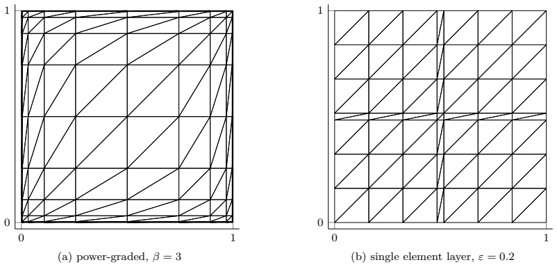
A counterexample to Theorem 2 would be a sequence of two-dimensional conforming nondegenerate simplicial meshes satisfying the paper's assumptions for which $N\left(1+|\ln(N|\omega_{\min}|)|\right)\lambda_{\min}(A)$ tends to zero; the single-element-layer family is a concrete candidate to test. The three-dimensional analogue compares $\lambda_{\min}(A)$ with $\left(\sum_i |\omega_i|^{-1/2}\right)^{-2/3}$ on meshes with highly uneven patch volumes.
Extended reading notes
Core claim
The central discovery is that the smallest eigenvalue of the stiffness matrix for Lagrangian $P_m$ finite elements on a conforming nondegenerate simplicial mesh is bounded from below, with constants independent of the mesh, by an expression in the nodal patch volumes: for $d \ge 3$, $\lambda_{\min}(A) \gtrsim \left(\sum_{i\in\mathcal{N}} |\omega_i|^{1-d/2}\right)^{-2/d}$; for $d=2$, $\lambda_{\min}(A) \gtrsim N^{-1}\left(1+|\ln(N|\omega_{\min}|)|\right)^{-1}$. Here $|\omega_i|$ is the volume of the patch of simplices containing node $i$, and $N$ is the number of degrees of freedom. The derivation goes through the $H^1$ energy, Poincaré and Sobolev inequalities, norm equivalence on the reference simplex, and Hölder's inequality, with the novel step of reassembling element contributions by nodal patches before applying Hölder. In three and more dimensions the bound is equivalent to $N^{-1}$ times a power of a Hölder mean of the ratios $|\tilde{\omega}|/|\omega_i|$, so it reacts to how irregular the patch volumes are, not to the worst element. In two dimensions the optimal choice of the $L^p$ exponent yields the logarithmic factor involving the smallest patch volume.
Load-bearing premise
The whole argument rests on one mesh-independent constant: on a standard reference simplex, the ratio between the $L^p$ size of a finite element function and the $\ell^p$ size of its list of nodal values must stay bounded as the exponent $p$ grows. This is true for a fixed polynomial degree, but if that ratio grew with $p$, the two-dimensional logarithmic bound would fail for extremely small patch volumes.
Editorial extensions
If this is right
- In $d \ge 3$, the bound $\lambda_{\min}(A) \gtrsim \left(\sum_i |\omega_i|^{1-d/2}\right)^{-2/d}$ holds on meshes with arbitrary anisotropy and local refinement, so local mesh irregularity alone cannot drive the smallest eigenvalue to zero faster than the patch-volume sum dictates.
- In two dimensions, for practical mesh sizes where $N|\omega_{\min}|$ is not astronomically small, the logarithmic factor is $O(1)$, so the smallest eigenvalue behaves like $N^{-1}$.
- The new estimate removes the factor depending on the maximal volume ratio of neighboring elements that appeared in the earlier regularity-dependent bound, and replaces elementwise averaging with patch-based averaging in the previous arbitrary-mesh bound.
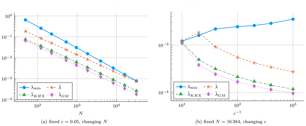
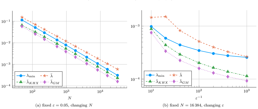
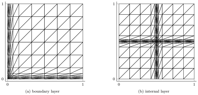
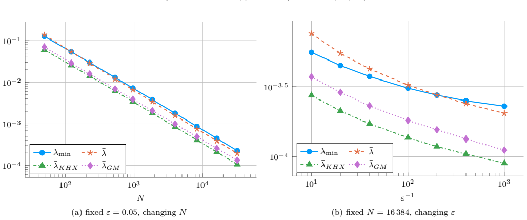
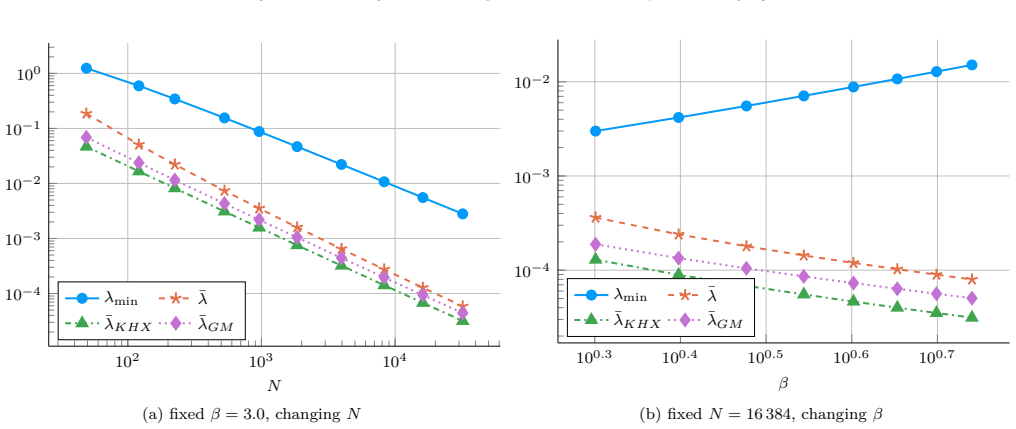
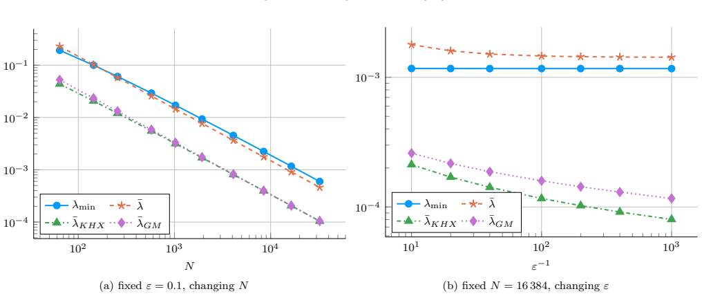
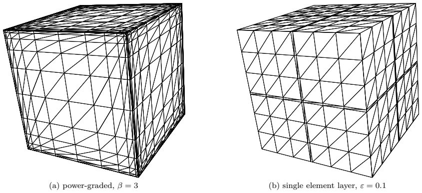
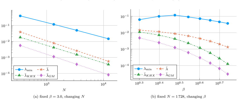
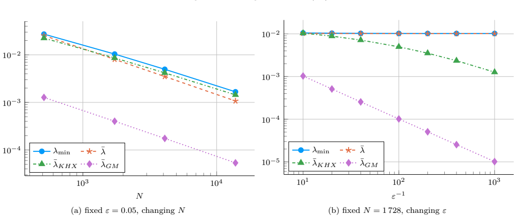
- For the mesh families tested in the paper—Shishkin, Bakhvalov, power-graded, and single-element-layer meshes—the new bound stays close to the exact smallest eigenvalue, while the earlier estimates underestimate it by factors that grow with mesh anisotropy.
- The proof uses only uniform ellipticity, Poincaré and Sobolev inequalities, and conforming nondegenerate simplicial meshes, so the same statement applies to any elliptic problem satisfying those conditions.
Reading between the lines
- A practical rule follows from the bound: what controls the smallest eigenvalue is the distribution of patch volumes, so mesh generators and preconditioners that keep patch volumes balanced should control conditioning better than those that merely keep element shapes regular. The paper does not discuss preconditioning.
- The proof technique—choosing the $L^p$ exponent before applying Hölder and then reassembling by patches—is generic enough that it may carry over to other finite element spaces, mass matrices, or nonconforming methods; testing that transfer is a natural next step.
- If the two-dimensional logarithmic dependence on $|\omega_{\min}|$ is not optimal, then on meshes with one very small patch but otherwise regular volumes the exact $\lambda_{\min}(A)$ should stay close to $C N^{-1}$ even when $N|\omega_{\min}|$ becomes very small; the paper leaves this as an open direction.
Signed reviews
Editorial analysis
A structured set of objections, weighed in public.
Referee Report
Summary. The paper proves new lower bounds on the smallest eigenvalue of the finite element stiffness matrix for Lagrangian P_m elements on arbitrary conforming simplicial meshes in d ≥ 2, without any mesh regularity assumptions. In d ≥ 3 (Theorem 1, Eq. (7)) the bound is λ_min(A) ≳ (∑_{i ∈ N} |ω_i|^{1-d/2})^{-2/d}, and in d = 2 (Theorem 2, Eq. (11)) it is λ_min(A) ≳ N^{-1}(1 + |ln(N |ω_min|)|)^{-1}. The proof combines the Poincaré inequality, the Sobolev embedding (or its two-dimensional variant), the norm equivalence on the reference element, and Hölder's inequality, and avoids the local comparability Assumption 1 of Graham and McLean. Numerical experiments on Shishkin, Bakhvalov, power-graded, and single-element-layer meshes compare the new bound with the bounds of Graham–McLean and Kamenski–Huang–Xu, showing that the new bound is sharper and less dependent on mesh nonuniformity.
Significance. If correct, the main result settles a clean open point: the smallest eigenvalue of the stiffness matrix is controlled, up to constants independent of the mesh, solely by the number of degrees of freedom and the distribution of patch volumes, with no shape-regularity or local-comparability condition. The derivation is self-contained and parameter-free in the sense that no quantity in the bound is fitted from data, and the numerical section provides concrete evidence of sharpness on several challenging mesh families. The principal technical caveat is the implicit assumption that the reference-element norm-equivalence constant is uniform in the exponent p, which is needed in Theorem 2 because p is chosen to grow with the mesh; this assumption is true for fixed polynomial degree and should be stated explicitly. Overall this is a clean and useful contribution to the conditioning literature.
major comments (1)
- [Section 4, proof of Theorem 2, Eq. (12)] The step labeled 'Norm equivalence ... yields' in Eq. (12) implicitly assumes that the norm-equivalence constant between ||u_h ∘ F_K||_{L^p(ˆK)} and ||u_K||_{l^p} is independent of p, or at least bounded uniformly in p for fixed polynomial degree m. In Theorem 2, p = max{2, |ln(N|ω_min|)|} depends on the mesh and can be arbitrarily large, so the final logarithmic bound (11) requires this uniformity. The author should add a short justification (e.g., via Hölder's inequality and the finite-dimensional equivalence of L^∞ and L^2 on the reference simplex) to make this step explicit. This is the only load-bearing point in the paper that I found to be implicit rather than fully stated.
minor comments (4)
- [Section 4, after Eq. (13)] The phrase 'provides the largest lower bound' is not literally correct, since the specific choice p = max{2, |ln(N|ω_min|)|} does not always maximize the factor appearing in (13); it merely yields a valid lower bound of the stated form. Consider rewording to 'provides a lower bound of the stated form.'
- [Remark 4] There are several typographical errors in this remark: 'bewteen' should be 'between', 'exmaples' should be 'examples', 'reguarity' should be 'regularity', and 'it not clear' should be 'it is not clear'.
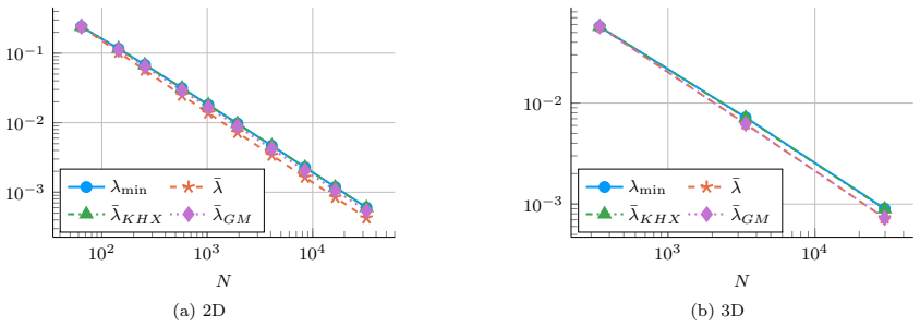
- [Section 5, Eqs. (14) and (15)] The constants in the numerical estimates are chosen empirically so that the bounds coincide with the exact λ_min on uniform meshes; this is disclosed in the text but could be repeated in the figure captions to prevent readers from interpreting the plotted curves as uncalibrated theoretical predictions.
- [Section 5, Eq. (14b)] The factors M and H appear in Eq. (14b) without being defined in Section 5; the reader must refer back to Assumption 1. Adding a one-line reminder after Eq. (14) would improve readability.
Circularity Check
No circularity: the lower bounds are derived from standard inequalities and are not fitted, self-referential, or equivalent to their inputs.
full rationale
The central claims (Theorem 1 for d >= 3 and Theorem 2 for d = 2) are self-contained derivations. Starting from the ellipticity condition (5), the proof bounds u^T A u below via Poincare and Sobolev inequalities, finite-dimensional norm equivalence on the reference simplex, and Holder's inequality. None of these inputs contains the target bound: the norm-equivalence step is a standard property of the fixed polynomial-degree space P_m on the reference element, and the constants involved are independent of the mesh and, for fixed m, bounded uniformly in p >= 2, so the p = |log(N|omega_min|)| choice in Theorem 2 is safe. The paper's citations to [11] and [8] are used only for comparison and for proof inspiration, not as load-bearing premises: the inequality chain is written out in the paper. The numerical experiments explicitly calibrate unknown constants so that plotted estimates coincide with the exact eigenvalue on uniform meshes (Figure 3 caption: 'Constants are chosen such that the bounds coincide with the exact value on uniform meshes'), and this calibration is a display choice, not part of the proof or a prediction. There is no self-definitional reduction, no fitted parameter renamed as a prediction, and no uniqueness or ansatz imported from the author's prior work. The only fragile-looking step, the p-dependence of the reference-element norm-equivalence constant, is uniform for fixed polynomial degree, so it does not threaten the derivation.
Assumptions & free parameters
assumptions (7)
- standard math Poincaré inequality on bounded Lipschitz domain Omega for H^1_0(Omega) functions
- standard math Sobolev embedding H^1(Omega) subset L^{2d/(d-2)}(Omega) for d >= 3 and H^1(Omega) subset L^p(Omega) for all finite p in d = 2
- standard math Norm equivalence on the reference simplex between the L^q norm of a P_m function and the l^q norm of its nodal coefficients
- standard math Hölder's inequality with exponents p = d/(d-2), q = d/2 (and the corresponding 2D choice)
- domain assumption Uniform positive definiteness of the diffusion matrix D(x), d_min I <= D(x) <= d_max I
- domain assumption Conforming, nondegenerate simplicial mesh with affine mappings F_K from a unit reference simplex
- domain assumption Bounded Lipschitz domain Omega
Cite this review
Pith. "Pith review of Sharp bounds on the smallest eigenvalue of finite element equations with arbitrary meshes without regularity assumptions." pith.science (2026). https://pith.science/paper/WH4UTKRW
@misc{pith2026190803460,
  author       = {Pith},
  title        = {Pith review of: Sharp bounds on the smallest eigenvalue of finite element equations with arbitrary meshes without regularity assumptions},
  year         = {2026},
  howpublished = {\url{https://pith.science/paper/WH4UTKRW}},
  note         = {Machine review of arXiv:1908.03460}
}
abstract
A proof for the lower bound is provided for the smallest eigenvalue of finite element equations with arbitrary conforming simplicial meshes. The bound has a similar form as the one by Graham and McLean [SIAM J. Numer. Anal., 44 (2006), pp. 1487--1513] but doesn't require any mesh regularity assumptions, neither global nor local. In particular, it is valid for highly adaptive, anisotropic, or non-regular meshes without any restrictions. In three and more dimensions, the bound depends only on the number of degrees of freedom $N$ and the H\"older mean $M_{1-d/2} (\lvert \tilde{\omega} \rvert / \lvert \omega_i \lvert)$ taken to the power $1-2/d$, $\lvert \tilde{\omega} \rvert$ and $\lvert \omega_i \rvert$ denoting the average mesh patch volume and the volume of the patch corresponding to the $i^{\text{th}}$ mesh node, respectively. In two dimensions, the bound depends on the number of degrees of freedom $N$ and the logarithmic term $(1 + \lvert \ln (N \lvert \omega_{\min} \rvert) \rvert)$, $\lvert \omega_{\min} \rvert$ denoting the volume of the smallest patch. Provided numerical examples demonstrate that the bound is more accurate and less dependent on the mesh non-uniformity than the previously available bounds.
Figures

Figures from the paper (11 more)

Reference graph
Works this paper leans on
-
[1]
M. Ainsworth, W. McLean, and T. Tran. The conditioning of boundary element equations on locally refined meshes and preconditioning by diagonal scaling. SIAM J. Numer. Anal., 36(6):1901–1932, 1999
work page 1901
-
[2]
M. Ainsworth, W. McLean, and T. Tran. Diagonal scaling of stiffness matrices in the Galerkin boundary element method. ANZIAM J., 42(1):141–150, 2000. Papers in honour of David Elliott on the occasion of his sixty-fifth birthday
work page 2000
-
[3]
R. E. Bank and L. R. Scott. On the conditioning of finite element equations with highly refined meshes.SIAM J. Numer. Anal., 26(6):1383–1394, 1989
work page 1989
-
[4]
J. Bezanson, A. Edelman, S. Karpinski, and V.B. Shah. Julia: a fresh approach to numerical computing.SIAM Rev., 59(1):65– 98, 2017
work page 2017
-
[5]
Q. Du, D. Wang, and L. Zhu. On mesh geometry and stiffness matrix conditioning for general finite element spaces.SIAM J. Numer. Anal., 47(2):1421–1444, 2009
work page 2009
-
[6]
A. Ern and J.-L. Guermond.Theory and practice of finite ele- ments, volume 159 ofApplied Mathematical Sciences. Springer- Verlag, New York, 2004
work page 2004
-
[7]
I. Fried. Bounds on the spectral and maximum norms of the finite element stiffness, flexibility and mass matrices.Internat. J. Solids and Structures, 9:1013–1034, 1973
work page 1973
-
[8]
I. G. Graham and W. McLean. Anisotropic mesh refinement: the conditioning of Galerkin boundary element matrices and simple preconditioners. SIAM J. Numer. Anal., 44(4):1487–1513, 2006
work page 2006
Show all 14 references
-
[9]
StabilityofexplicitRunge- Kutta methods for high order finite element approximation of linear parabolic equations
W.Huang, L.Kamenski, andJ.Lang. StabilityofexplicitRunge- Kutta methods for high order finite element approximation of linear parabolic equations. In Numerical mathematics and advanced applications—ENUMATH 2013, volume 103 ofLect. Notes Comput. Sci. Eng., pages 165–173. Springe...
2013
-
[10]
Kamenski and W
L. Kamenski and W. Huang. A study on the conditioning of finite element equations with arbitrary anisotropic meshes via a density function approach. J. Math. Study, 47(2):151–172, 2014
2014
-
[11]
Kamenski, W
L. Kamenski, W. Huang, and H. Xu. Conditioning of finite element equations with arbitrary anisotropic meshes. Math. Comp., 83:2187–2211, 2014
2014
-
[12]
Shewchuk
J.R. Shewchuk. What is a good linear finite element? Interpola- tion, conditioning, anisotropy, andqualitymeasures, 2002.https: //www.cs.berkeley.edu/~jrs/jrspapers.html#quality
2002
-
[13]
Zhu and Q
L. Zhu and Q. Du. Mesh-dependent stability for finite element approximations of parabolic equations with mass lumping.J. Comput. Appl. Math., 236(5):801–811, 2011
2011
-
[14]
Zhu and Q
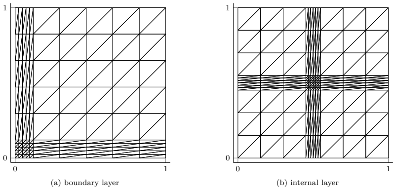
L. Zhu and Q. Du. Mesh dependent stability and condition number estimates for finite element approximations of parabolic problems. Math. Comp., 83(285):37–64, 2014. 6 0 1 0 1 (a) boundary layer 0 1 0 1 (b) internal layer Figure 4: Shishkin meshes,ε= 0.05 (2D). 102 103 104 10−4 ...
2014
Reviewed August 14, 2026 · model on record in the stance chip above.
Discussion (0). Continue with ORCID to comment.