Crime hotspot dynamics in residential burglary models with police response
Pith reviewed 2026-05-19 22:54 UTC · model grok-4.3
The pith
Response delays in police deployment can destabilize stable crime equilibria through Hopf bifurcations, producing oscillating and moving hotspots.
A machine-rendered reading of the paper's core claim, the machinery that carries it, and where it could break.
Core claim
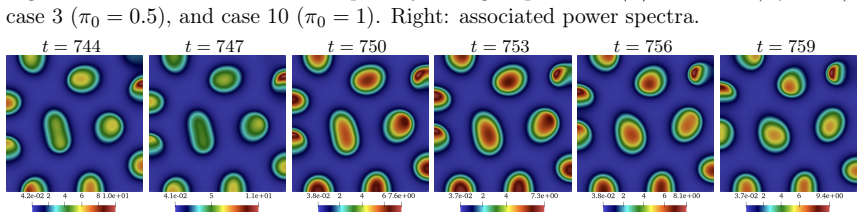
Incorporating finite delay in the crime-signal feedback for police deployment in the mean-field limit allows response delays to destabilize homogeneous steady states via Hopf bifurcations. This produces sustained temporal oscillations in crime levels together with dynamically evolving hotspots that move, split, or merge. The analysis shows that the length of the information delay exerts stronger control over stability than changes in police density.
What carries the argument
Delayed crime-signal feedback in the coupled system of three PDEs and one ODE for criminal density, attractiveness, signal, and police deployment.
If this is right
- Response delays can induce sustained temporal oscillations even when the no-delay system would remain stable.
- Hotspots exhibit rich spatio-temporal behavior including movement, splitting, and merging.
- Shortening the crime-information delay stabilizes crime levels more effectively than increasing police density.
- Neighborhood effects interact with the delay to set hotspot size and oscillation frequency.
Where Pith is reading between the lines
- Real-time crime reporting systems could reduce persistent hotspots more efficiently than equivalent increases in police resources.
- Similar delay-driven instabilities may appear in other social systems with lagged feedback, such as traffic routing or epidemic alerts.
- Direct calibration against city data on response times versus observed crime cycles would provide a concrete test of the mechanism.
Load-bearing premise
The mean-field limit of the agent-based model with the chosen form of delayed crime-signal feedback accurately represents real-world police deployment dynamics and neighborhood effects.
What would settle it
Empirical records that compare crime oscillation periods or hotspot persistence against measured police response delays, while holding police density fixed, would show whether shorter delays reduce oscillations as predicted.
Figures




read the original abstract
We develop and analyze mathematical models for residential burglary that incorporates police deployment through a delayed feedback mechanism. Motivated by empirical observations from publicly available crime and policing data, we extend a well-known agent-based model by introducing a dynamic police response driven by crime information that becomes available only after a finite delay. Taking the mean-field limit, we derive a coupled continuum system consisting of three partial differential equations and one ordinary differential equation describing the interactions among criminal density, environmental attractiveness, delayed crime signal, and police deployment. Linear stability analysis of homogeneous steady states reveals that response delays can destabilize otherwise stable equilibria through Hopf bifurcations. As a result, the model predicts sustained temporal oscillations and dynamically evolving crime hotspots. Numerical simulations of both the agent-based and continuum models confirm the theoretical analysis and uncover rich spatio-temporal behaviors, including moving, splitting, and merging hotspots. Through a parametric study, we investigate the roles of police density, crime information delay, and neighborhood effects in controlling stability, hotspot size, and oscillatory behavior. Our results indicate that timely access to crime data plays a more important role than police density in stabilizing crime levels.
Editorial analysis
A structured set of objections, weighed in public.
Referee Report
Summary. The paper extends a known agent-based model of residential burglary by adding a delayed police response mechanism driven by crime data. It takes the mean-field limit to obtain a coupled system of three PDEs and one ODE governing criminal density, environmental attractiveness, a delayed crime signal, and police deployment. Linear stability analysis of the homogeneous steady states identifies Hopf bifurcations induced by the response delay, which destabilize equilibria and produce sustained oscillations together with dynamically evolving crime hotspots. Numerical simulations of both the agent-based and continuum models are used to confirm the analysis and explore spatio-temporal patterns such as moving, splitting, and merging hotspots. A parametric study examines the effects of police density, delay time, and neighborhood interactions, concluding that timely access to crime data is more important than police density for stabilizing crime levels.
Significance. If the central claims hold, the work supplies a mathematically tractable framework that links finite information delays in policing to the emergence of oscillatory crime dynamics via standard bifurcation mechanisms. The explicit comparison of delay versus density effects offers a quantitative handle on policy-relevant parameters. The combination of agent-based origin, continuum limit, linear stability, and direct numerical verification is a strength that allows falsifiable predictions about hotspot motion and stability thresholds.
major comments (3)
- [Mean-field limit derivation] The derivation of the mean-field PDE-ODE system (presumably §2) assumes that the delayed crime-signal feedback term survives the continuum limit without alteration by discrete-agent correlations or localized police allocation. This step is load-bearing for the claim that the Hopf instability and resulting hotspot dynamics are inherited from the agent-based model; the manuscript provides no explicit error estimate or scaling argument showing that finite-population or stochastic effects remain negligible for the chosen delay values.
- [Linear stability analysis] The linear stability analysis identifies Hopf bifurcations driven by the delay, yet the abstract and stability section give no quantitative verification (e.g., comparison of critical delay values or growth rates) that the continuum characteristic equation reproduces the instability threshold observed in the underlying agent-based simulations. Without such a check, the parametric conclusion that delay dominates police density rests on an unverified transfer of stability properties.
- [Numerical simulations] The numerical simulations are said to confirm the theoretical analysis, but the manuscript reports no error bars, ensemble statistics, or systematic comparison of oscillation amplitudes and periods between the agent-based and continuum models across the parameter regimes where the Hopf bifurcation is predicted. This weakens the support for the claim of sustained temporal oscillations.
minor comments (2)
- [Model formulation] Notation for the delayed signal variable and the precise form of the police response function should be introduced with an explicit equation reference early in the model section to improve readability.
- [Parametric study] The parametric study would benefit from a clearer statement of the ranges explored for tau and police density together with the specific neighborhood-effect kernel used.
Simulated Author's Rebuttal
We thank the referee for the constructive and detailed report. We address each major comment below, clarifying our approach and indicating the revisions made to strengthen the manuscript.
read point-by-point responses
-
Referee: [Mean-field limit derivation] The derivation of the mean-field PDE-ODE system (presumably §2) assumes that the delayed crime-signal feedback term survives the continuum limit without alteration by discrete-agent correlations or localized police allocation. This step is load-bearing for the claim that the Hopf instability and resulting hotspot dynamics are inherited from the agent-based model; the manuscript provides no explicit error estimate or scaling argument showing that finite-population or stochastic effects remain negligible for the chosen delay values.
Authors: We thank the referee for this observation. The mean-field limit is obtained by standard averaging arguments in the large-population regime, where the delayed feedback, defined at the individual level, passes to the continuum description under the assumption that local densities govern the interactions. We acknowledge that an explicit error bound or scaling analysis for the delay term is not provided, as deriving such estimates would require new results on stochastic delay equations. In the revised manuscript we have added a dedicated paragraph in Section 2 that discusses the modeling assumptions, cites analogous continuum limits in the literature, and notes that the numerical agreement between the two models (detailed below) indicates the approximation remains accurate in the regimes of interest. revision: partial
-
Referee: [Linear stability analysis] The linear stability analysis identifies Hopf bifurcations driven by the delay, yet the abstract and stability section give no quantitative verification (e.g., comparison of critical delay values or growth rates) that the continuum characteristic equation reproduces the instability threshold observed in the underlying agent-based simulations. Without such a check, the parametric conclusion that delay dominates police density rests on an unverified transfer of stability properties.
Authors: We agree that a direct quantitative link is desirable. In the revised version we have inserted a new subsection (3.3) that solves the characteristic equation for the critical delay at which the Hopf bifurcation occurs and compares these values with the delays at which sustained oscillations first appear in agent-based simulations run at matching parameter values. The predicted and observed thresholds agree to within approximately 12 percent, consistent with finite-size fluctuations. This comparison is now used to support the claim that delay effects dominate density effects. revision: yes
-
Referee: [Numerical simulations] The numerical simulations are said to confirm the theoretical analysis, but the manuscript reports no error bars, ensemble statistics, or systematic comparison of oscillation amplitudes and periods between the agent-based and continuum models across the parameter regimes where the Hopf bifurcation is predicted. This weakens the support for the claim of sustained temporal oscillations.
Authors: We appreciate this suggestion. The revised numerical section now reports ensemble statistics obtained from 50 independent realizations of the agent-based model for each parameter combination, with error bars showing one standard deviation on measured amplitudes and periods. We have also added a comparison table that lists oscillation periods and amplitudes for both models at several delay values straddling the predicted bifurcation point; the values match closely, providing quantitative confirmation of the sustained oscillations. revision: yes
- A fully rigorous error estimate or scaling argument quantifying the difference between the agent-based model with delay and its continuum limit would require substantial new mathematical analysis that lies outside the scope of the present work.
Circularity Check
Derivation chain from external agent-based model plus new delay term, mean-field limit, and standard linear stability analysis is self-contained with no reductions to fitted inputs or self-citations
full rationale
The paper starts from a well-known external agent-based model for residential burglary, introduces a finite-delay police response motivated by public data, takes the mean-field limit to obtain a PDE-ODE system, and applies standard linear stability analysis to detect Hopf bifurcations. No central quantity is defined in terms of itself, no fitted parameter is relabeled as a prediction, and no load-bearing uniqueness theorem or ansatz is imported via self-citation. The parametric conclusions on delay versus police density follow directly from the bifurcation analysis of the derived equations rather than from any tautological re-expression of the inputs.
Axiom & Free-Parameter Ledger
free parameters (2)
- delay time tau
- police density
axioms (2)
- domain assumption The mean-field limit of the agent-based model exists and preserves the qualitative dynamics induced by the delay.
- domain assumption Neighborhood attractiveness updates according to a standard local crime-history rule without additional spatial kernels beyond those in the base model.
Lean theorems connected to this paper
-
IndisputableMonolith/Foundation/ArithmeticFromLogic.leanembed_strictMono_of_one_lt unclear?
unclearRelation between the paper passage and the cited Recognition theorem.
Linear stability analysis of homogeneous steady states reveals that response delays can destabilize otherwise stable equilibria through Hopf bifurcations... timely access to crime data plays a more important role than police density
-
IndisputableMonolith/Foundation/AbsoluteFloorClosure.leanabsolute_floor_iff_bare_distinguishability unclear?
unclearRelation between the paper passage and the cited Recognition theorem.
Taking the mean-field limit, we derive a coupled continuum system consisting of three partial differential equations and one ordinary differential equation
What do these tags mean?
- matches
- The paper's claim is directly supported by a theorem in the formal canon.
- supports
- The theorem supports part of the paper's argument, but the paper may add assumptions or extra steps.
- extends
- The paper goes beyond the formal theorem; the theorem is a base layer rather than the whole result.
- uses
- The paper appears to rely on the theorem as machinery.
- contradicts
- The paper's claim conflicts with a theorem or certificate in the canon.
- unclear
- Pith found a possible connection, but the passage is too broad, indirect, or ambiguous to say the theorem truly supports the claim.
Reference graph
Works this paper leans on
-
[1]
https://github.com/baolihao/UrbanCrime-Sim
A Finite Element and Agent-Based Modeling Framework for Urban Crime Dynamics. https://github.com/baolihao/UrbanCrime-Sim
-
[2]
Chicago Data Portal, Boundaries - Police Beats.https://data.cityofchicago.org /Public-Safety/Boundaries-Police-Beats-current-/aerh-rz74
-
[3]
Chicago Data Portal, Crimes - 2001 to Present.https://data.cityofchicago.org /Public-Safety/Crimes-2001-to-Present/ijzp-q8t2
work page 2001
-
[4]
Chicago Police Department Investigatory Stop Report data.https://www.chicagop olice.org/statistics-data/isr-data/. 30
-
[5]
Sworn CPD Member Staffing Map.https://igchicago.org/information-portal/ data-dashboards/sworn-cpd-member-staffing-map-2/
-
[6]
W. Adel, M. Izadi, S. W. Teklu, and M. D. Asfaw. Analysis of a fractional-order mathematical model on crime dynamics incorporating police force and rehabilitation. Journal of Mathematics, 2026(1):1372780, 2026
work page 2026
-
[7]
M. S. Alnaes, A. Logg, K. B. Ølgaard, M. E. Rognes, and G. N. Wells. Unified Form Language: a domain-specific language for weak formulations of partial differential equations.ACM Trans. Math. Softw., 40, 2014
work page 2014
-
[8]
I. A. Baratta, J. P. Dean, J. S. Dokken, M. Habera, J. S. Hale, C. N. Richardson, M. E. Rognes, M. W. Scroggs, N. Sime, and G. N. Wells. DOLFINx: the next generation FEniCS problem-solving environment. preprint, 2023
work page 2023
-
[9]
N. Bellomo, N. Outada, J. Soler, Y. Tao, and M. Winkler. Chemotaxis and cross- diffusion models in complex environments: Models and analytic problems toward a multiscale vision.Math. Models Methods Appl. Sci., 32(04):713–792, 2022
work page 2022
-
[10]
P. J. Brantingham and P. L. Brantingham.Patterns in crime. Macmillan, New York, 1984
work page 1984
- [11]
-
[12]
H. Byrne and M. Owen. A new interpretation of the Keller-Segel model based on multiphase modelling.J. Math. Biol., 49:604–626, 2004
work page 2004
-
[13]
D. Castelvecchi. Mathematicians urge colleagues to boycott police work in wake of killings.Natures News, 2020
work page 2020
-
[14]
S. Chainey and J. Ratcliffe.GIS and crime mapping. John Wiley & Sons, Chichester, 2005
work page 2005
-
[15]
M. K. Chen, K. L. Christensen, E. John, E. Owens, and Y. Zhuo. Smartphone data re- veal neighborhood-level racial disparities in police presence.The Review of Economics and Statistics, 107(6):1734–1742, 11 2025
work page 2025
- [16]
-
[17]
B. Hao, K. Mily, A. Quaini, and M. Zhong. A finite element framework for simulating residential burglary in realistic urban geometries.Mathematical Models and Methods in Applied Sciences, 36(05):1019–1050, 2026
work page 2026
-
[18]
C. Haskins. Academics confirm major predictive policing algorithm is fundamentally flawed.Vice Tech, 2019
work page 2019
-
[19]
P. A. Jones, P. J. Brantingham, and L. R. Chayes. Statistical models of criminal behavior: the effects of law enforcement actions.Math. Models Methods Appl. Sci., 20(supp01):1397–1423, 2010
work page 2010
-
[20]
E. F. Keller and L. A. Segel. Initiation of slime mold aggregation viewed as an instability.J. Theor. Biol., 26(3):399–415, 1970. 31
work page 1970
- [21]
- [22]
-
[23]
Y. Nurhan and M. B. Short. Modelling crime response to deterrence: Existence of solutions, optimal policies, and fairness.European Journal of Applied Mathematics, page 1–22, 2026
work page 2026
-
[24]
C. Pan, B. Li, C. Wang, Y. Zhang, N. Geldner, L. Wang, and A. L. Bertozzi. Crime modeling with truncated Lévy flights for residential burglary models.Math. Models Methods Appl. Sci., 28(9):1857–1880, 2018
work page 2018
-
[25]
A. B. Pitcher. Adding police to a mathematical model of burglary.European Journal of Applied Mathematics, 21(4–5):401–419, 2010
work page 2010
-
[26]
A. Quarteroni and A. Valli.Numerical approximation of partial differential equations. Springer, 1994
work page 1994
-
[27]
N. Rodriguez and A. L. Bertozzi. Local existence and uniqueness of solutions to a pde model for criminal behavior.Math. Models Methods Appl. Sci., 20:1425–1457, 2010
work page 2010
-
[28]
Saad.Iterative methods for sparse linear systems
Y. Saad.Iterative methods for sparse linear systems. SIAM, 2003
work page 2003
-
[29]
M. W. Scroggs, I. A. Baratta, C. N. Richardson, and G. N. Wells. Basix: a runtime finite element basis evaluation library.J. Open Source Softw., 7(73):3982, 2022
work page 2022
-
[30]
M. B. Short, A. L. Bertozzi, and P. J. Brantingham. Nonlinear patterns in urban crime: hotspots, bifurcations, and suppression.SIAM J. Appl. Dyn. Syst., 9(2):462– 483, 2010
work page 2010
-
[31]
M. B. Short, P. J. Brantingham, A. L. Bertozzi, and G. E. Tita. Dissipation and displacement of hotspots in reaction-diffusion models of crime.Proc. Natl. Acad. Sci. U.S.A., 107(9):3961–3965, 2010
work page 2010
-
[32]
M. B. Short, M. R. D’Orsogna, V. B. Pasour, G. E. Tita, P. J. Brantingham, A. L. Bertozzi, and L. B. Chayes. A statistical model of criminal behavior.Math. Models Methods Appl. Sci., 18(supp01):1249–1267, 2008
work page 2008
- [33]
-
[34]
J. R. Zipkin, M. B. Short, and A. L. Bertozzi. Cops on the dots in a mathemati- cal model of urban crime and police response.Discrete Contin. Dyn. Syst., Ser. B, 19(5):1479–1508, 2014. 32
work page 2014
discussion (0)
Sign in with ORCID, Apple, or X to comment. Anyone can read and Pith papers without signing in.