REVIEW 3 major objections 5 minor 24 references
Modeling and Analysis of Phase-locked loops: a non reductionist approach
T0 review · 3 major / 5 minor · reviewed 2026-08-12 · deepseek-v4-flash
Pith's one-line read A four-state model of the phase-locked loop maps synchronization and desynchronization regions directly, without phase-error reduction.
desk verdict The non-reductionist idea is sensible, but the phase estimator in Eq. (8) is wrong, so the synchronization maps and noise results are unsupported as written. read the letter →
The pith
A machine-rendered reading of the paper's core claim, the machinery that carries it, and where it could break.
The reading
What carries the argument
The carrying object is the four-state state-space model in Eq. (6): $\dot{x}_1=x_2$, $\dot{x}_2=-a_0x_1-a_1x_2+K_d z_1 u(t)$, $\dot{z}_1=z_2$, and $\dot{z}_2=-[\omega_0+K_v(b_0x_1+b_1x_2)]^2 z_1$. It couples a second-order loop filter, states $x_1,x_2$, with a VCO oscillator, states $z_1,z_2$, through the multiplicative phase detector. The work this does is to keep the loop's actual oscillating signals as state variables, so high-frequency components survive in the filter output and noise can be inserted at circuit-accessible points. The companion machinery is the phase-recovery formula $\psi_o=\tan^{-1}(z_2/z_1)$ and the metrics in Eq. (12), which turn simulation traces into synchronization maps.
What would settle it
Recompute the parameter maps of Figures 10-12 with a phase estimate that accounts for the VCO amplitude and frequency, for example $\psi_o = \operatorname{atan2}(-z_2/(\omega_0+K_v v_c), z_1)$ with unwrapping, and compare the locations and floor levels of the synchronization regions; if the blue plateaus move or change shape, the reported boundaries are artifacts of the Eq. (8) estimator rather than properties of the model.
Extended reading notes
Core claim
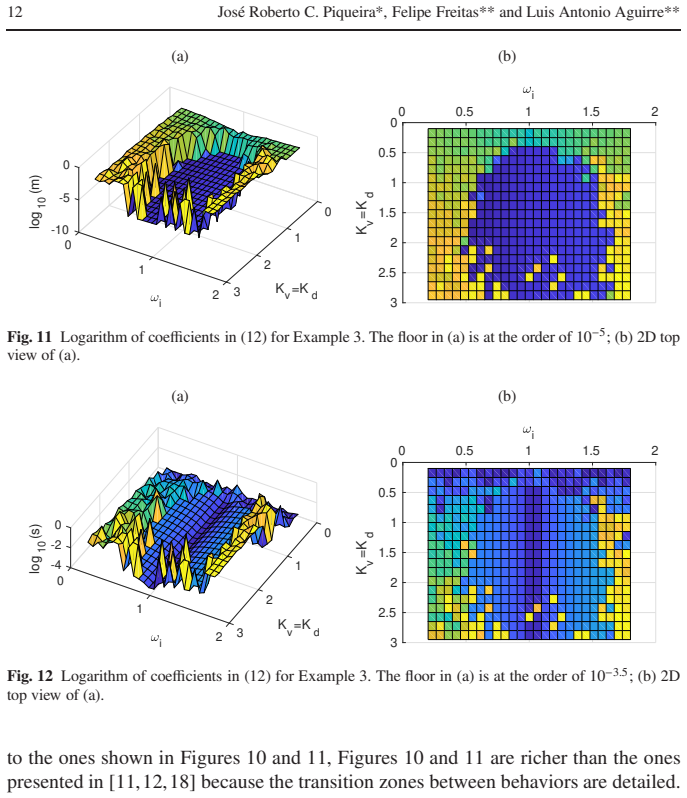
The central claim is that the four-state model in Eq. (6), with filter states $x_1,x_2$ and oscillator states $z_1,z_2$, represents a third-order PLL node more faithfully than phase-reduction models because the multiplier phase detector $v_d = K_d z_1 u(t)$ and the VCO frequency $\omega_{\rm inst}=\omega_0+K_v(b_0x_1+b_1x_2)$ are kept as they are, with no averaging away of high-frequency terms and no assumption of equal input and output frequencies. The output phase is estimated as $\psi_o = \tan^{-1}(z_2/z_1)$, and synchronization performance is quantified by frequency-entrainment error $f$, phase-error magnitude $e$, mean absolute phase-error derivative $m$, and its standard deviation $s$. Parameter scans over input frequency $\omega_i$ and loop gain $K_d=K_v$ produce maps whose flat floors mark the capture and lock-in regions. The maps show a broad synchronization band around $\omega_i\approx\omega_0$ with gain between 1 and 2, and noisy runs show that noise shrinks and asymmetrizes the locking region while roughly preserving its floor level.
Load-bearing premise
The load-bearing premise is that the output phase recovered from the oscillator states through Eq. (8) is the actual VCO phase; since every synchronization metric in Eq. (12) is built from this estimate, a systematic error in that recovery would shift the capture and lock-in boundaries in Figures 10-12.
Editorial extensions
If this is right
- Capture and lock-in ranges become visible as floors in parameter maps of $f$, $m$, and $s$, so they can be found by numerical integration instead of analytical bifurcation or phase-plane calculations.
- Because the model does not assume ideal filtering, design choices such as filter bandwidth and roll-off can be tested directly for their effect on residual high-frequency ripple in the control voltage.
- Different VCO structures, such as adding an integral term to the frequency control, can be simulated without changing the modeling framework, enabling zero steady-state frequency error designs.
- Noise can be injected at the VCO central frequency or at the input, and Monte Carlo runs can be used to check how much the synchronization region shrinks or becomes asymmetric.
- The resulting maps agree in broad terms with earlier bifurcation-based studies of third-order PLLs while exposing transition zones between synchronized and desynchronized regimes in more detail.
Reading between the lines
- Implicit in the paper, the same parameter-scan strategy could be applied to networks of PLL nodes by coupling several copies of Eq. (6), replacing analytical network stability conditions with searchable maps.
- The synchronization maps are only as trustworthy as the phase estimate: redoing Figures 10-12 with a corrected phase recovery such as $\operatorname{atan2}(-z_2/\omega_{\rm inst}, z_1)$ with unwrapping could shift the reported boundaries, so the regions should be treated as qualitative until that check is done.
- The apparent stabilizing effect visible in the noisy $s$ map is worth testing separately, since $s$ measures variability of the phase-error derivative rather than synchronization itself; varying the noise variance in a controlled sweep would show whether the effect is genuine or an artifact of the metric.
Editorial analysis
A structured set of objections, weighed in public.
Referee Report
Summary. The paper proposes a four-state 'non reductionist' state-space model of a phase-locked loop, comprising a harmonic-oscillator VCO, a second-order loop filter, and a multiplicative phase detector. It uses this model to estimate the VCO output phase via Eq. (8) and defines synchronization metrics f, e, m, s in Eq. (12) to map capture/lock-in regions in parameter space, with and without noise. The claimed contribution is that these maps provide design-relevant synchronization boundaries without the usual phase-reduction assumptions.
Significance. If the model and phase estimates were sound, the paper would offer a useful numerical design tool for third-order PLLs, including nonideal filtering and noise. The manuscript provides explicit state equations, a clear simulation protocol, and parameter sweeps without fitting parameters to a target result; those are genuine strengths. The central quantitative claims, however, rest on a phase estimator that is mathematically inconsistent with the oscillator state equations, and on a VCO representation that is not the standard FM relation when the control voltage varies. No experimental or circuit-level validation is provided, so the practical claims rest entirely on the simulation model, which as written is not reliable.
major comments (3)
- [Section 2, Eq. (8); Section 3, Eqs. (10)-(12)] The phase estimator psi_o(t)=tan^{-1}(z2/z1) is not the output phase of the oscillator (1). If z1=A cos(phi) and z2=-A omega_inst sin(phi), then psi_o=tan^{-1}(-omega_inst tan(phi)), not phi. When unwrapped, this estimate has a mean slope of approximately -omega_inst, so in a locked state with phi approximately omega_i t the average Omega_o in Eq. (11) would be about -omega_i and the frequency-entrainment measure f in Eq. (12) would be of order 2, rather than the 1e-3 floor reported in Figure 10. Consequently, the small e-dot values in Figure 6, the thresholds in Eq. (10), and all parameter-space maps in Figures 10-12 and 15-17 are not reproduced by the formulas as stated. A corrected four-quadrant estimator such as atan2(-z2/omega_inst, z1) with unwrapping would have to be specified and the simulations regenerated.
- [Section 2, Eqs. (1)-(2)] The text states that the oscillator (1) has solution z1=A cos(omega_inst t) and that this represents an FM VCO. This is only valid if omega_inst is constant. When vc(t) varies, the solution of (1) is not A cos(omega_inst t); writing z1=A cos(phi) and differentiating shows that (1) requires phi_ddot=0 and phi_dot=omega_inst, which is incompatible with a time-varying control voltage. The correct FM phase relation is phi(t)=integral_0^t [omega0+Kv vc(tau)] d tau. The model as written is therefore not the standard FM VCO used in PLL analysis, and the physical interpretation in the surrounding text is not supported.
- [Section 3, Eq. (9) and model (6)] Equation (9) introduces an integral term Ki times the integral of vc in omega_inst, but no corresponding state is present in the proposed state-space model (6). Example 2 states that the VCO is simulated with (2) 'and with an integral term', and Example 3 uses Ki=0.22 to produce Figures 10-12. The simulations therefore are not of the model (6) that the paper derives and claims to analyze; they are of a different dynamical system whose equations are not given. This is a consistency gap between the mathematical model and the numerical evidence.
minor comments (5)
- [Section 3, Example 3] The parameter grid is described only as yielding 520 combinations; the number of points in each dimension and the step sizes should be stated for reproducibility.
- [Section 4] The implementation of noise in the central frequency omega0 and in the input u(t) within the state equations (6) is not specified (e.g., continuous-time white noise, sample-and-hold noise, or random initial perturbations). A precise stochastic definition is needed to reproduce the Monte Carlo results.
- [Section 2, after Eq. (2)] The expression z1=A cos[(omega0+Kv vc(t))t] is dangerous notation: for time-varying vc(t) the argument should be the integral of (omega0+Kv vc(tau)) d tau, not the product (omega0+Kv vc(t))t.
- [Figure 6 and Eq. (12)] The derivative e_dot in Eq. (12) is computed from a phase estimate with branch cuts; the unwrapping procedure used to obtain Figures 10-12 should be stated explicitly, because the reported floors depend on it.
- [Section 1 and Section 5] The claim that the state-space model 'takes into account the nonlinearity of the sine function' is not precisely tied to Eq. (5), where the phase detector is a product of two sinusoidal signals; the relationship between this product and the usual sine phase-detector characteristic should be clarified.
Circularity Check
No circularity: the state-space model and synchronization metrics are independently defined and the results are numerical observations, not fitted or self-citation-derived predictions.
full rationale
The paper's derivation chain is self-contained. The state-space model in Eq. (6) is assembled directly from the oscillator equations (1)-(2), the filter realization (4), and the multiplicative phase detector (5); none of these equations is defined in terms of the synchronization metrics f, e, m, and s introduced later in Eq. (12). The metrics are post-processing measures applied to simulated signals, and the paper sweeps parameter values and reports observed floors, so there is no parameter fitted to a target result and later relabeled as a prediction. The self-citations [10], [12], [14], and [18] are used for context, prior reductionist results, and comparisons, but the load-bearing model and its numerical analysis do not reduce to those citations. The thresholds and definitions in Eqs. (10)-(12) are attributed to external synchronization literature [16, 23], not to prior work by the authors. Even if Eq. (8) is mathematically questionable as a phase estimator, that would be a correctness or validity concern, not circularity, because the measured phase is not defined as the synchronization result it is used to evaluate. No step satisfies the requirement of exhibiting a reduction by construction or a fitted input renamed as a prediction.
Assumptions & free parameters
free parameters (2)
- Loop filter coefficients (a0, a1, b0, b1) =
1/3, 1/2, 1/3, 1/12
- VCO integral gain Ki in Eq. (9) =
0.5 in Example 2, 0.22 in Example 3
assumptions (4)
- domain assumption Phase detector output is the exact product vd = Kd z1(t) u(t)
- ad hoc to paper VCO obeys the harmonic-oscillator equation with instantaneous frequency omega(t) = omega0 + Kv vc(t), and its solution is A cos(omega(t) t)
- ad hoc to paper Synchronization can be judged by the floor levels of the metrics f, m, and s defined in Eq. (12)
- ad hoc to paper The phase of the VCO output is recovered by psi_o = atan(z2/z1)
Cite this review
Pith. "Pith review of Modeling and Analysis of Phase-locked loops: a non reductionist approach." pith.science (2026). https://pith.science/paper/WOZXB7EE
@misc{pith2026241117759,
  author       = {Pith},
  title        = {Pith review of: Modeling and Analysis of Phase-locked loops: a non reductionist approach},
  year         = {2026},
  howpublished = {\url{https://pith.science/paper/WOZXB7EE}},
  note         = {Machine review of arXiv:2411.17759}
}
read the original abstract
Phase-locked loop (PLL), conceived in 1932 by H. Bellescize, has been the basic electronic component in the development of communication technology from the early analog radio receptors to modern digital civil and military facilities. Traditionally, the analysis is conducted by modeling the dynamical behavior of phase and frequency errors, hence following a phase reduction approach. One of the main goals of the present work is to describe and investigate the dynamics of a PLL node by representing it in full state-space, here called non reductionist model, without the usual design simplifications i.e., considering different input and output frequencies and not neglecting the higher frequencies components generated in the phase detection process. On the one hand, this approach complicates the use of analytical tools but on the other hand it permits an efficient numerical approach that can be used for precise definition of regions in parameters space that show the boundaries between synchronization and non synchronization regimes, even when noise is considered. Results show that the PLL node can be simulated in a more realistic way using the state-space model and that a number of design-relevant aspects can now be investigated numerically.
Figures
Reference graph
Works this paper leans on
-
[1]
de Bellescize H., La reception synchrone L’Onde electriq ue, changed to revue de l’electricit´ e et de l’electronique, vol. 11 (1932), pp. 230-240
work page 1932
-
[2]
Staszewski R.B., Balsara P .T., Phase-domain all-digita l phase-locked loop IEEE Transactions on Cir- cuits and Systems II, Exp Briefs, 52 (3) (2005), pp. 159-163
work page 2005
-
[3]
Alvarez M.A., Spagnolini U., Distributed time and carrie r frequency synchronization for dense wire- less networks, IEEE Transactions on Signal and Information Processing over Networks, 4 (4) (2018), pp. 683-696
work page 2018
-
[4]
Lindsey W.C. Synchronization systems in communication a nd control (1st ed), Prentice Hall, En- giewood Cliffs, NJ: USA (1972)
work page 1972
- [5]
- [6]
-
[7]
Bregni S. A historical perspective on telecommunication s network synchronization, IEEE Communi- cations Magazine, 36 (6) (1998), pp. 158-166
work page 1998
-
[8]
Bregni S. Synchronization of digital telecommunication s networks, (1st ed), John Wiley & Sons, Ltd., West Sussex-UK (2002)
work page 2002
Show all 24 references
-
[9]
Phase-locked loops (6th ed), McGraw Hill, New Y o rk (2007)
Best R.E. Phase-locked loops (6th ed), McGraw Hill, New Y o rk (2007)
2007
-
[10]
Piqueira J.R.C., de Godoi A.C.B., Clock signal distribu tion with second order nodes: Design hints ISA Transactions, 115(2021), pp. 124-142
2021
-
[11]
066101-2–066101-20
Dandapathak M., Chakraborty S., Studies on of phase erro r oscillations in a class of third-order optical phase locked loop and its e ffect on a slave optical phase locked loop, Optical Engineerin g, 61(6) (2022), pp. 066101-2–066101-20
2022
-
[12]
Piqueira J.R.C., Hopf bifurcation and chaos in a third-o rder phase-locked loop, Communications in Nonlinear Science and Numerical Simulation, 42 (2017), pp. 178-186
2017
-
[13]
Nakao H., Phase reduction approach to synchronisation o f nonlinear oscillators, Contemporary Physics 57(2016), pp. 188-214
2016
-
[14]
50(2003), pp
Piqueira, J.R.C., Monteiro, L.H.A., Considering secon d-harmonic terms in the operation of the phase detector for second-order phase-locked loop, IEEE Tr ansactions on Circuits and Systems I, v. 50(2003), pp. 805-809, 2003
2003
-
[15]
Hsieh, G. C. and Hung, J. C. Phase-locked loop techniques - a survey. IEEE Transactions on Industrial Electronics, 43(6) (1996), pp. 609-615
1996
-
[16]
V ., Kurths, J., and Zhou, C., Synchronization in Oscillatory Networks, Springer, Berlin (2007)
Osipov, G. V ., Kurths, J., and Zhou, C., Synchronization in Oscillatory Networks, Springer, Berlin (2007)
2007
-
[17]
2454-2464
Leonov G.A., Kuznetsov N.V ., Y uldashev M.V ., Y uldashevR.V ., Hold-in, pull-in, and lock-in ranges of PLL circuits: Rigorous mathematical definitions and limi tations of classical theory, IEEE Transac- tions on Circuits and Systems I: Regular Papers, 62 (10) (201 5), pp. 245...
-
[18]
Piqueira, J. R. C., Using bifurcations in the determinat ion of lock in ranges for third-order phase- locked loops, Communications in Nonlinear Science Numeric al Simulation, 14 (5) (2009), pp. 2328–2335. (https: //doi.org/10.1016/j.cnsns.2008.06.012)
2009 doi
-
[19]
Clusella P ., Politi A., Noise-induced stabilization of collective dynamics, Physical Review E 95(2017), 062221
2017
-
[20]
Viterbi, Phase-Locked Loop Dynamics in the Presence o f Noise by Fokker-Planck Techniques, Proceedings of the IEEE, 12 (1963), pp
A. Viterbi, Phase-Locked Loop Dynamics in the Presence o f Noise by Fokker-Planck Techniques, Proceedings of the IEEE, 12 (1963), pp. 1737-1753
1963
-
[21]
4113 - 4116, International Conference on Elec tric Information and Control Engineering (2011)
Xu, X., Huihua, L., Ao, S., Design of low phase noise and fa st locking PLL frequency synthesizer, 2011 International Conference on Electric Information and Control Engineering, ICEICE 2011 - Pro- ceedings, pp. 4113 - 4116, International Conference on Elec tric Information and...
2011
-
[22]
2040 - 2044
Ripani, B., Modenini, A., Montorsifellow, G., Digital P LLs for Phase Noise Channels: A Concept Based on the Tikhonov Distribution, IEEE Signal Processing Letters, 31(2024), pp. 2040 - 2044. (DOI: 10.1109/LSP .2024.3432048)
2024
-
[23]
G., Pikovsky, A
Rosenblum, M. G., Pikovsky, A. S., and Kurths, J., Phase s ynchronization of chaotic oscillators, Phys- ical Review Letters, 76(11)(1996), pp. 1804-1807
1996
-
[24]
Moschas, F., Stiros, S., PLL bandwidth and noise in 100 Hz GPS measurements, GPS Solutions, 19(2015), pp. 173–185
2015
Reviewed August 12, 2026 · model on record in the stance chip above.
Discussion (0). Continue with ORCID to comment.