Summary Statistics of Large-scale Model Outputs for Observation-corrected Outputs

Atlanta Chakraborty; Julie Bessac

REVIEW 5 major objections 7 minor 50 references

Summary Statistics of Large-scale Model Outputs for Observation-corrected Outputs

T0 review · 5 major / 7 minor · reviewed 2026-08-06 · deepseek-v4-flash

Challenge this review Re-run · record.json Download PDF Read on arXiv ↗

Pith's one-line read Sig-PCA shows that bias-correcting physics-based model outputs can be done from low-dimensional path-signature summaries instead of full gridded fields, yielding corrected probability distributions and spatial correlations.

desk verdict A sensible and clearly written Sig-PCA pipeline for bias correction, but the central out-of-sample claim is untested because all evaluation uses the stations used to train the corrective network. read the letter →

arxiv 2506.15845 v1 pith:WPAEJBL2 submitted 2025-06-18 stat.ME stat.APstat.COstat.ML

Atlanta Chakraborty , Julie Bessac This is my paper

classification stat.MEstat.APstat.COstat.ML MSC 62M3062H2562M1068T07

keywords pathsignaturebiascorrectionprincipalcomponentanalysisdeepkrigingneuralnetworkspatio-temporalstatisticssurfacetemperaturewindspeed

verification ladder T0 review T1 audit T2 compute T3 formal

The pith

A machine-rendered reading of the paper's core claim, the machinery that carries it, and where it could break.

The reading

Physics-based models such as reanalysis and numerical weather prediction generate fields that are biased and large enough to be hard to store and move, while observations are sparse. This paper proposes Sig-PCA, a pipeline that extracts low-dimensional path-signature summary statistics from the full model grid, reduces them by PCA, and trains neural networks on these summaries to reconstruct the model field and add observation-based corrections. The authors demonstrate on surface temperature and surface wind data that the corrected fields match the probability distributions, spatial correlation, and spectral content of the observations far better than the raw model output, and also better than an EOF-based summary benchmark. The significance is that bias correction need not ingest the entire gridded field; only a compressed summary has to be moved and processed.

What carries the argument

The central object is the path signature of the model field at each grid location: for a time series $x$, the depth-$N$ signature stacks iterated integrals $\int_{t_0\le u_1\le\cdots\le u_d\le t_1} dx_{i_1,u_1}\cdots dx_{i_d,u_d}$ for $d=1,\dots,N$, evaluated over the seven sub-windows produced by dyadic windowing at depth 3. These signatures encode temporal displacement (depth 1) and signed areas between locations (depth 2) at multiple scales. PCA then reduces the signature space to the components explaining 99.5% of the variance, and the resulting vectors feed two fully connected networks: a reconstruction network that recovers the full grid from a small fraction of training locations, and a corrective network that predicts observation-minus-reconstruction discrepancies. Multi-resolution Wendland radial basis functions from deep kriging, together with spatial coordinates, are the mechanism that transfers corrections from the sparse observation stations to the rest of the grid.

What would settle it

Hold out one-third of the observation stations entirely from training, then compare corrected model fields at those held-out stations against observations; if the corrected fields are no closer to observations than the raw model output, the claim of spatially transferable correction fails. A second check is to withhold a full season of the year and see whether reconstructed and corrected fields reproduce the observed spectral and spatial correlation structure in that season.

Watch

Extended reading notes

Core claim

The paper's central claim is that a two-stage neural-network procedure operating only on reduced representations of physics-based model outputs can produce observation-corrected fields whose probability distributions and space-time correlation structures align with observations. In the first stage, a reconstruction network recovers the full model grid from path-signature summaries computed over seven dyadic time windows and projected onto principal components retaining 99.5% of the variance; in the second stage, a corrective network learns the discrepancy between observations and the nearest reconstructed gridpoints, with deep kriging basis functions carrying the corrections to unobserved locations. The authors state that this is the first bias-correction method built from reduced representations of model outputs rather than from their full gridded fields. On NLDAS surface temperature, training on 4% of the gridpoints yields about 11.05% reconstruction error and a 70.09% improvement over raw model RMSE at observation stations; on WRF surface wind, the reconstruction error is about 13.63% with a 51.61% improvement, and depth-2 signatures help capture the noisier wind field.

Load-bearing premise

The method assumes that the compressed summary statistics, a few hundred numbers per time window, still carry enough information to rebuild the full model field and to extend corrections to the roughly 96% of gridpoints without observations, and the paper supports this only with in-sample reconstruction errors and correction improvements rather than held-out data.

Editorial extensions

If this is right

Corrected fields inherit the model's spatial support while matching observed statistics, so analyses that need full-coverage, observation-consistent fields can use the corrected grid rather than raw model output.
The method reduces the amount of model data that must be moved for bias correction to a few hundred summary components, opening the door to correcting fields where full outputs cannot be stored or transferred.
The two-stage design, reconstructing the model first and then learning observation discrepancies, gives better spatial correlation alignment than directly predicting observations, according to the paper's comparisons.
Because only summaries of model outputs are needed, the approach can be applied to datasets with different smoothness and different model-to-observation ratios, as demonstrated by the temperature and wind experiments.

Reading between the lines

Editorial extensions of the paper, not claims the author makes directly.

If signatures were computed only at adaptively chosen locations instead of every gridpoint, the method could run entirely in situ; the paper's k-centroid experiment suggests that the quality of such a reduction would depend strongly on the smoothness of the field.
The 99.5% variance threshold and the depth-3 windowing are natural tuning knobs; an explicit sweep over signature depth and retained variance would reveal whether even smaller summaries suffice for a given field.
Because the corrective network is trained on station discrepancies, its errors should scale with station density; a natural stress test is to thin the observation network and measure the degradation of corrected spatial correlations.
The smoother temperature field showed larger reconstruction-error differences between signature summaries and clustering-based summaries, suggesting that the choice of reduced representation matters most in fields with strong spatial structure.

Share X Bluesky LinkedIn Reddit HN

Editorial analysis

A structured set of objections, weighed in public.

Desk editor's note, referee report, and a circularity audit.

Desk Editor's Note

read the letter

The short version: a useful, clearly written proposal for bias-correcting climate model outputs via path-signature summaries, but all the headline metrics are computed on the same stations used to train the corrective network, so the paper's main generalization claim is not yet supported.

What is actually new: the idea of treating path signatures as summary statistics for physics-based model outputs, then feeding PCA-reduced signatures into reconstruction and correction networks, appears to be novel. The paper shows that the reduced representation can reconstruct NLDAS temperature and WRF wind fields to about 11-14% RMSE using 4% of the gridpoints, and that the corrected fields match observation distributions and spatial correlations better than raw model output. The method is assembled from known parts, but the combination is new. The authors also provide code and a sensitivity analysis on training gridpoint fraction. That is real work and worth acknowledging.

Where the soft spots are: the evaluation is systematically in-sample. The corrective network is trained on the differences between observations and reconstructed model output at the observation stations (Algorithm 1, Step 5), and the same stations are used to compute all reported improvement metrics, Wasserstein distances, QQ plots, and correlation curves. The network can, in principle, memorize station-specific biases, and nothing in the paper rules that out. The full-grid maps and correlation curves do not separate trained from untrained stations, so the reader cannot tell whether the correction transfers to unobserved locations. A spatial holdout---train on half the stations, evaluate on the other half---would answer this directly.

The comparison with EOF is also uneven: Sig-PCA retains 135 components for temperature and 41 for wind, while EOF retains 11 and 17. Both retain 99.5% of variance, but the number of components differs by an order of magnitude, so the comparison is not apples-to-apples. There is also a subtle leakage in the reconstruction evaluation: PCA is computed on signatures from all gridpoints, so the inputs for a held-out location contain global information about that location. That makes the reconstruction RMSE an optimistic measure of generalization.

None of these problems are load-bearing in the sense that the method is incoherent. They are fixable with a proper holdout evaluation and a matched-component baseline or clear justification for the different truncation levels. The paper is an honest demonstration of a plausible pipeline, but it is not yet a demonstration of out-of-sample correction.

Bottom line: readers working on statistical post-processing or in-situ compression of large climate model outputs will find the framework worth knowing about. As is, I would not use the quantitative improvement numbers in a citation. But this deserves serious peer review: the idea is sensible, the writing is clear, and the validation gap is addressable.

Referee Report

5 major / 7 minor

Summary. The paper proposes Sig-PCA, a framework for correcting gridded physics-based model outputs using sparse observations. The method computes depth-1 (and selectively depth-2) path signatures over hierarchical dyadic windows for each model gridpoint, applies PCA to the signature space to retain 99.5% variance, and then trains two neural networks: a reconstruction network that maps PCA-reduced signatures (plus coordinates and deep-kriging basis functions) to model values at a subset of gridpoints, and a corrective network that learns the discrepancy between observations and reconstructed model values at nearby gridpoints. The corrected field is obtained by adding the predicted correction to the reconstructed field over the full grid. The approach is demonstrated on NLDAS surface temperature (with LCD stations) and WRF surface wind speed (with ASOS stations), and is compared against an EOF-based reduction baseline. The paper also includes sensitivity analyses, seasonal diagnostics, QQ plots, spatial correlation curves, and spectral comparisons.

Significance. The proposed idea is timely and potentially useful: combining unsupervised signature summaries of large model outputs with neural-network-based spatial correction could reduce the computational burden of bias correction and post-processing. The paper provides code, two real-data applications with different statistical properties, and a fairly comprehensive set of validation diagnostics. However, the central generalization claim — that corrections learned at a sparse set of observation stations extend to unobserved locations — is currently supported only by in-sample evaluation: all correction metrics are computed at the same stations used to train the corrective network. The comparison against EOF is also confounded by a large asymmetry in the number of retained components. If the authors add proper out-of-sample (held-out station) validation and a more balanced benchmark, the work could make a solid contribution to the applied statistics and climate post-processing literature.

major comments (5)

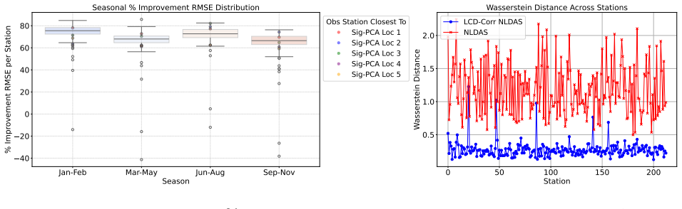
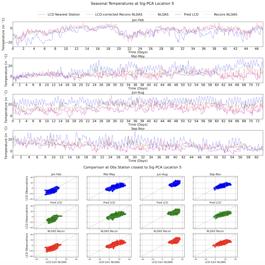
[Sections 4.3 and 5.3; Algorithm 1 Steps 5-7] The central generalization claim of the paper — that corrections learned at roughly 4% of gridpoints extend to unobserved locations — is not supported by the reported evaluation. The corrective NN in Algorithm 1 Step 5 is trained on Corr_obs = F_obs - C_recon_obs' at the LCD/ASOS stations, and all quantitative metrics in Sections 4.3 and 5.3 (% improvement RMSE, 1-Wasserstein distances, QQ plots, spatial correlation curves, spectra) are computed at precisely those same stations. High scores could therefore reflect memorization of station-specific biases rather than spatially transferable corrections. The authors should add a held-out evaluation: either spatial cross-validation (train on a subset of stations, test on the rest) or temporal holdout, and report metrics separately for trained versus untrained stations.
[Sections 2.5, 4.2, 5.2] The comparison against the EOF baseline is asymmetric. Sig-PCA retains 135 principal components for temperature and 41 for wind, while the EOF baseline retains 11 and 17 components, respectively (Sections 4.2 and 5.2). With roughly an order of magnitude more degrees of freedom, the Sig-PCA reconstruction and correction would be expected to fit the training data better regardless of the summary-statistic quality. To support the claim that Sig-PCA outperforms EOF, the authors should either match the number of retained components across methods (e.g., plot performance versus number of components for both) or otherwise control for representation capacity.
[Section 2.4, Algorithm 1 Steps 2-4] The reconstruction RMSE (11.05% for temperature, 13.63% for wind) is presented as a measure of how well the method reconstructs the full model field from a small fraction of gridpoints, but it is not a clean out-of-sample test. The PCA in Step 2 is fit on path signatures from all gridpoints, so the reduced representation supplied to the reconstruction NN at a held-out location already contains information from that location through the global principal-component loadings. The reported RMSE is therefore a compression-reconstruction error, not a test of generalization to locations whose data were never used. This should be stated explicitly, and if spatial generalization is the goal, the PCA should be fit only on the training subset or a leave-location-out scheme should be adopted.
[Sections 1 and 6] The claim that this is the first attempt to bias-correct physics-based model outputs from reduced representations is too strong given the cited literature. Guinness and Hammerling (2018) use Fourier coefficients as summary statistics for statistical compression and conditional emulation of climate model output, which is closely related in spirit to correcting outputs from reduced summaries, and model output statistics (MOS) have long operated on dimension-reduced predictors. The authors should either soften this claim or provide a precise delimitation of what distinguishes the present approach from these earlier reduced-representation correction methods.
[Sections 2.2, 4.1, 5.1] The sufficiency of the chosen summary statistics is not established. The window depth is fixed at dw=3 and the signature depth at N=1 for temperature and at N=1 plus partial depth-2 for wind; no sensitivity analysis is reported for these choices. Since the entire approach rests on the claim that depth-1/depth-2 path signatures over seven dyadic windows, after PCA retention of 99.5% variance, retain the information needed for correction, the authors should provide an evaluation across at least one or two alternative settings (e.g., dw=2 or N=2 applied consistently) and show that the correction quality is not critically dependent on the specific hyperparameter values.

minor comments (7)

[Section 2.2] The sentence "we set the window depth to dw = 3, meaning the data is divided into dw + 1 sub-windows" is incorrect; the total number of sub-windows is 2^{dw+1}-1 = 7, not 4.
[Section 2.4] The description of the reconstruction network inputs is ambiguous: the phrase "using summary statistics from the full grid as inputs" could mean either the global PCA-reduced signature vector for each time window or per-location summary values. Please clarify the exact input tensor shape for both the reconstruction and correction networks.
[Section 4.2] The statement "The value of x is selected based on practical constraints and the desired percentage RMSE" is not consistent with the later choice of x=4%, which is justified by the number of LCD stations; please clarify the actual selection rationale.
[Section 6] The phrase "while working a reduced representation" should read "while working with a reduced representation."
[Sections 4.2 and 5.3] The aggregate improvement values 70.09% and 51.61% are reported without specifying how the per-station % improvement RMSE values are averaged across stations and seasons; please define the aggregation.
[Abstract] The phrase "different ratios of model to observational data" is vague; specify what ratio is meant (e.g., number of gridpoints to observation stations, or sample sizes).
[Section 3.2] The moving-window filter applied to the ASOS wind data is not described; state the window length and type, and how the hourly picks were made after filtering.

Circularity Check

2 steps flagged · score 6.0 of 10

Headline correction metrics are computed at the same observation stations used to train the corrective network; reconstruction error is evaluated over training gridpoints with PCA fit on the full grid.

fitted input called prediction [Algorithm 1, Step 5; Section 4.3; Section 5.3]
"Use the PCA-reduced representation as input to train the corrective NN to learn the corrections, Corr obs = Fobs − C recon obs′ for obs′ locations that are closest to the obs locations."

The corrective network's training target at each station is the residual between the observations Fobs and the reconstructed field at the nearest gridpoint. The paper's headline validation metrics—% improvement RMSE, 1-Wasserstein distance, QQ plots, and station-level spatial correlations—are then all evaluated at those same LCD/ASOS stations. Consequently, the reported improvements measure in-sample fit of the correction network rather than its ability to transfer corrections to unobserved locations. The central claim that corrections learned at roughly 4% of gridpoints extend to the full grid is therefore not independently tested; the evaluation set is the training set by construction.
fitted input called prediction [Section 4.2 (reconstruction sensitivity); Algorithm 1, Steps 3–4]
"After reconstructing the entire grid, the error between the original and reconstructed NLDAS is evaluated across all gridpoints."

The reconstruction network is trained on x% of the model gridpoints, while its inputs are PCA-reduced signatures computed from the full grid of model outputs. The reported reconstruction RMSE is averaged over all gridpoints, including the x% used as training targets, and the PCA basis is itself estimated from all gridpoints, including any locations one might wish to treat as held out. The reconstruction error is therefore not a clean out-of-sample measure of whether the reduced signature representation generalizes to unseen gridpoints; the fitted PCA representation already contains information from the evaluation locations.

full rationale

Sig-PCA's construction is not self-definitional: path signatures and PCA are computed from model outputs alone, and the corrective residual is defined from observations; there is no equation in which the claimed prediction equals its input by definition. The circularity lies in evaluation. Algorithm 1 Step 5 trains the corrective NN on Corr_obs = F_obs − C_recon at the observation stations, and Sections 4.3/5.3 score the corrected field against the same LCD/ASOS stations. The % improvement RMSE and 1-Wasserstein distances therefore quantify in-sample fit, not spatial transfer. Similarly, the reconstruction experiments evaluate RMSE over all gridpoints, including training targets, while PCA is fit on all gridpoints, so the reported 11.05%/13.63% errors are not clean holdout estimates. No load-bearing self-citation chain is present; Bessac et al. (2018) supplies data and Chen et al. (2022) supplies deep kriging, and neither is invoked to forbid alternatives. The method has independent content, but its central generalization claim is currently supported only by in-sample validation, giving a partial circularity score of 6.

Assumptions & free parameters 6 free parameters · 5 assumptions · 0 invented entities

The central claim rests on standard statistical tools (signatures, PCA, kriging, neural networks) and on treating observations as ground truth. The main ad hoc element is the choice of hyperparameters, which are tuned on the same data and not independently validated.

free parameters (6)

Signature depth N = 1 for temperature, 2 for wind
Chosen based on data properties; only first-order integrals for temperature, second-order for wind at selected locations (Sections 4.1, 5.1).
Dyadic window depth d_w = 3
Yields 7 sub-windows; authors state going beyond 3 is unreliable with daily/hourly data (Section 2.2).
PCA variance threshold = 99.5%
Determines number of principal components kept: 135 for temperature, 41 for wind (Sections 4.1, 5.1).
Training gridpoint fraction x = 4%
Mimics observation density; sensitivity analysis shows error stabilizes only near 20% (Section 4.2).
Deep kriging Wendland bandwidth = 2.5 times knot spacing
Taken directly from Chen et al. (2022) without re-estimation (Section 2.4).
NN architecture hyperparameters = 7 layers (512 to 16) for temperature; 2 hidden layers (128, 64) for wind; learning rate 0.01; 500 epochs
Reported without systematic tuning or validation set (Sections 4.2, 5.2).

assumptions (5)

standard math Path signatures determine a path up to tree-like equivalence and provide sufficient summary statistics for sequential data.
Invoked in Section 2.1 to justify using signatures as summary statistics; based on Lyons theory.
standard math Karhunen-Loeve expansion allows a spatial process to be represented by a finite linear combination of orthogonal basis functions.
Used to motivate deep kriging basis functions in Section 2.4.
domain assumption The neural networks can approximate the reconstruction and correction mappings from the reduced features.
Implicit in Sections 2.4, 4.2, 5.2; no universal approximation or convergence guarantees are stated.
domain assumption Observations are treated as ground truth with negligible measurement error after temporal averaging.
Stated in Sections 3.1 and 3.2, where LCD and ASOS data are used as validation targets.
domain assumption Model outputs and observations are comparable after aligning temporal resolution (hourly means).
Section 3.1 mentions uniform one-hour intervals; Section 3.2 describes filtering and hourly picks.

how reviews work

0 comments

Cite this review

Pith. "Pith review of Summary Statistics of Large-scale Model Outputs for Observation-corrected Outputs." pith.science (2026). https://pith.science/paper/WPAEJBL2

@misc{pith2026250615845,
  author       = {Pith},
  title        = {Pith review of: Summary Statistics of Large-scale Model Outputs for Observation-corrected Outputs},
  year         = {2026},
  howpublished = {\url{https://pith.science/paper/WPAEJBL2}},
  note         = {Machine review of arXiv:2506.15845}
}

read the original abstract

Physics-based models capture broad spatial and temporal dynamics, but often suffer from biases and numerical approximations, while observations capture localized variability but are sparse. Integrating these complementary data modalities is important to improving the accuracy and reliability of model outputs. Meanwhile, physics-based models typically generate large outputs that are challenging to manipulate. In this paper, we propose Sig-PCA, a space-time framework that integrates summary statistics from model outputs with localized observations via a neural network (NN). By leveraging reduced-order representations from physics-based models and integrating them with observational data, our approach corrects model outputs, while allowing to work with dimensionally-reduced quantities hence with smaller NNs. This framework highlights the synergy between observational data and statistical summaries of model outputs, and effectively combines multisource data by preserving essential statistical information. We demonstrate our approach on two datasets (surface temperature and surface wind) with different statistical properties and different ratios of model to observational data. Our method corrects model outputs to align closely with the observational data, specifically enabling to correct probability distributions and space-time correlation structures.

Figures

Figures reproduced from arXiv: 2506.15845 by the authors.

**Figure 1.** Top network focuses on reconstructing model data from reduced signatures features, bottom network corrects errors between observations and gridded reconstructions. C represents the model outputs, F the observations, SS the path signatures summary statistics, DK the deep kriging basis functions, and (Lat, Lon) the spatial coordinates. The subscript Recon indicates the reconstruction process and mod the model gridpoi… view at source ↗

**Figure 2.** Left: The highlighted region in the Upper Midwest is enclosed within the bounding box. NOAA LCD stations are represented by squares, and the mean temperatures are displayed. Right: The region of interest surrounding Lake Michigan is depicted, with ASOS stations represented by squares. The temporal mean wind speed is displayed for all NWP simulation locations as well as ASOS observation sites. Cluster 2 in the regio… view at source ↗

**Figure 3.** Left: Most contributing Sig-PCA locations are shown in green circles. Selected 5 stations are highlighted with blue numbers for further analysis. Blue curves represent rivers. Red squares represent LCD observation locations. Right: Fluctuations of path signatures of the selected 5 top Sig-PCA locations across various sub-windows. insight into the underlying structure of the dataset. Each subplot corresponds to a dif… view at source ↗

Figures from the paper (22 more)

**Figure 4.** Figure 4: Path signatures variation across different sub-windows shown at the 5 [PITH_FULL_IMAGE:figures/full_fig_p014_4.png]

**Figure 5.** Figure 5: Sensitivity analysis of the percentage RMSE as a function of the per [PITH_FULL_IMAGE:figures/full_fig_p015_5.png]

**Figure 6.** Figure 6: Comparison of different approaches capturing the mean ( [PITH_FULL_IMAGE:figures/full_fig_p017_6.png]

**Figure 7.** Figure 7: Left: Seasonal % Improvement RMSE boxplot of LCD-corrected NLDAS and NLDAS with respect to LCD observation stations. The stations closest to the Sig-PCA locations are highlighted in different colors. Right: 1-Wasserstein distance across stations the LCD observations an…

**Figure 8.** Figure 8: Top: Comparison of different time series for Location 2 with the time series of nearest observation station, located very nearby. The LCD-corrected NLDAS is denoted in red, NLDAS in green, directly outputted LCD in purple and reconstructed NLDAS in cyan. Different rows…

**Figure 9.** Figure 9: Correlation as a function of distance between gridpoints. [PITH_FULL_IMAGE:figures/full_fig_p022_9.png]

**Figure 10.** Figure 10: Seasonal spectrum for spring (March-May) for the 5 selected locations [PITH_FULL_IMAGE:figures/full_fig_p023_10.png]

**Figure 11.** Figure 11: Grey dots mark the original NWP grid, the green circles show the top [PITH_FULL_IMAGE:figures/full_fig_p024_11.png]

**Figure 12.** Figure 12: NWP depth-2 path signatures of the five selected locations across vari [PITH_FULL_IMAGE:figures/full_fig_p026_12.png]

**Figure 13.** Figure 13: Fluctuations of path signatures of the NWP wind data at the five [PITH_FULL_IMAGE:figures/full_fig_p027_13.png]

**Figure 14.** Figure 14: NWP depth-2 path signatures of the selected locations across various [PITH_FULL_IMAGE:figures/full_fig_p028_14.png]

**Figure 15.** Figure 15: Comparison of different approaches of the mean ( [PITH_FULL_IMAGE:figures/full_fig_p030_15.png]

**Figure 16.** Figure 16: Comparison of different time series across all locations. The ASOS [PITH_FULL_IMAGE:figures/full_fig_p031_16.png]

**Figure 17.** Figure 17: Correlation as a function of the distance between gridpoints. Grey [PITH_FULL_IMAGE:figures/full_fig_p032_17.png]

**Figure 18.** Figure 18: Spectral analysis of the five selected stations across rows. The blue [PITH_FULL_IMAGE:figures/full_fig_p033_18.png]

**Figure 19.** Figure 19: Top: Comparison of different time series for Location 1 with the time series of nearest observation station. The LCD-corrected NLDAS is denoted in red, NLDAS in green, directly outputted LCD in purple and reconstructed NLDAS in cyan. Bottom: QQ-plot of outputs for dif…

**Figure 20.** Figure 20: Top: Comparison of different time series for Location 3 with the time series of nearest observation station. The LCD-corrected NLDAS is denoted in red, NLDAS in green, directly outputted LCD in purple and reconstructed NLDAS in cyan. Bottom: QQ-plot of outputs for dif…

**Figure 21.** Figure 21: Top: Comparison of different time series for Location 4 with the time series of nearest observation station. The LCD-corrected NLDAS is denoted in red, NLDAS in green, directly outputted LCD in purple and reconstructed NLDAS in cyan. Bottom: QQ-plot of outputs for dif…

**Figure 22.** Figure 22: Top: Comparison of different time series for Location 5 with the time series of nearest observation station. The LCD-corrected NLDAS is denoted in red, NLDAS in green, directly outputted LCD in purple and reconstructed NLDAS in cyan. Bottom: QQ-plot of outputs for dif…

**Figure 23.** Figure 23: Seasonal spectrum for winter (Jan-Feb) 42 [PITH_FULL_IMAGE:figures/full_fig_p042_23.png]

**Figure 24.** Figure 24: Seasonal spectrum for summer (June-Aug) 43 [PITH_FULL_IMAGE:figures/full_fig_p043_24.png]

**Figure 25.** Figure 25: Seasonal spectrum for winter (Sep-Nov) 44 [PITH_FULL_IMAGE:figures/full_fig_p044_25.png]

Discussion (0). Sign in to comment.

Reference graph

Works this paper leans on

50 extracted references · 44 canonical work pages

[1]

Abdul Qayyum, A. B., X. Luo, N. M. Urban, X. Qian, and B.-J. Yoon (2024). Implicit neural representations for simultaneous reduction and continuous reconstruction of multi-altitude climate data. In 2024 IEEE 34th International Workshop on Machine Learning for Signal Processing (MLSP) , pp.\ 1--6

work page 2024
[2]

Annau, N. J., A. J. Cannon, and A. H. Monahan (2023). Algorithmic Hallucinations of Near-Surface Winds: Statistical Downscaling with Generative Adversarial Networks to Convection-Permitting Scales . arXiv:2302.08720\/

arXiv 2023
[3]

Bailie, T., Y. S. Koh, N. Rampal, and P. B. Gibson (2024). Quantile-regression-ensemble: A deep learning algorithm for downscaling extreme precipitation. Proceedings of the AAAI Conference on Artificial Intelligence\/ 38\/ (20), 21914--21922

work page 2024
[4]

Constantinescu, and M

Bessac, J., E. Constantinescu, and M. Anitescu (2018). Stochastic simulation of predictive space–time scenarios of wind speed using observations and physical model outputs . The Annals of Applied Statistics\/ 12\/ (1), 432 -- 458

work page 2018
[5]

Cannon, A. J. (2018). Multivariate quantile mapping bias correction: an N-dimensional probability density function transform for climate model simulations of multiple variables . Climate dynamics\/ 50\/ (1), 31--49

work page 2018
[6]

Chen, W., Y. Li, B. J. Reich, and Y. Sun (2022). DeepKriging: Spatially Dependent Deep Neural Networks for Spatial Prediction . arXiv:2007.11972\/

work page Pith review arXiv 2022
[7]

Chevyrev, I. and A. Kormilitzin (2016). A Primer on the Signature Method in Machine Learning . arXiv:1603.03788\/

arXiv 2016
[8]

Christensen, H. and L. Zanna (2022, 12). Parametrization in weather and climate models

work page 2022

Show all 50 references

[9]

Cressie, N. (2015). Statistics for spatial data . John Wiley & Sons

2015
[10]

Cressie, N. and G. Johannesson (2008). Fixed-rank kriging for very large spatial data sets. Journal of the Royal Statistical Society: Series B (Statistical Methodology)\/ 70\/ (1), 209--226

2008
[11]

Danforth, C. M., E. Kalnay, and T. Miyoshi (2007). Estimating and correcting global weather model error. Monthly weather review\/ 135\/ (2), 281--299

2007
[12]

Daust, K. and A. Monahan (2024). Capturing Climatic Variability: Using Deep Learning for Stochastic Downscaling . arXiv:2406.02587\/

2024 arXiv
[13]

Di, S., J. Liu, K. Zhao, X. Liang, R. Underwood, Z. Zhang, M. Shah, Y. Huang, J. Huang, X. Yu, C. Ren, H. Guo, G. Wilkins, D. Tao, J. Tian, S. Jin, Z. Jian, D. Wang, M. H. Rahman, B. Zhang, S. Song, J. Calhoun, G. Li, K. Yoshii, K. Alharthi, and F. Cappello (2025). A survey on...

2025
[14]

Klein, L

Dutta, S., N. Klein, L. Tang, J. D. Wolfe, L. V. Roekel, J. J. Benedict, A. Biswas, E. Lawrence, and N. Urban (2021). In situ climate modeling for analyzing extreme weather events. In ISAV'21: In Situ Infrastructures for Enabling Extreme-Scale Analysis and Visualization , pp.\ 18--23

2021
[15]

Tasnim, T

Dutta, S., H. Tasnim, T. L. Turton, and J. Ahrens (2021). In Situ Adaptive Spatio-Temporal Data Summarization . In 2021 IEEE International Conference on Big Data (Big Data) , pp.\ 315--321

2021
[16]

Cannon, and S

Dyer, J., P. Cannon, and S. M. Schmon (2024). Approximate Bayesian Computation with Path Signatures . In The 40th Conference on Uncertainty in Artificial Intelligence

2024
[17]

Ramachandra, J

Ganguli, A., N. Ramachandra, J. Bessac, and E. Constantinescu (2024). Enhancing interpretability in generative modeling: Disentangled latent spaces in scientific datasets. Authorea Preprints\/

2024
[18]

Glahn, H. R. and D. A. Lowry (1972). The use of M odel O utput S tatistics ( MOS ) in objective weather forecasting. Journal of Applied Meteorology\/ 11\/ (8), 1203--1211

1972
[19]

Zhang, X

Gong, Q., C. Zhang, X. Liang, V. Reshniak, J. Chen, A. Rangarajan, S. Ranka, N. Vidal, L. Wan, P. Ullrich, N. Podhorszki, R. Jacob, and S. Klasky (2023). Spatiotemporally Adaptive Compression for Scientific Dataset with Feature Preservation – A Case Study on Simulation Data wi...

2023
[20]

Madaus, and C

Groenke, B., L. Madaus, and C. Monteleoni (2021). Climalign: Unsupervised statistical downscaling of climate variables via normalizing flows. In Proceedings of the 10th International Conference on Climate Informatics , CI2020, New York, NY, USA, pp.\ 60–66. Association for Com...

2021
[21]

Guinness, J. and D. Hammerling (2018). Compression and conditional emulation of climate model output. Journal of the American Statistical Association\/ 113\/ (521), 56--67

2018
[22]

Hannachi, A., I. T. Jolliffe, D. B. Stephenson, et al. (2007). Empirical orthogonal functions and related techniques in atmospheric science: A review. International journal of climatology\/ 27\/ (9), 1119--1152

2007
[23]

Dutta, H.-W

Hazarika, S., S. Dutta, H.-W. Shen, and J.-P. Chen (2019). CoDDA: A Flexible Copula-based Distribution Driven Analysis Framework for Large-Scale Multivariate Data . IEEE Transactions on Visualization and Computer Graphics\/ 25\/ (1), 1214--1224

2019
[24]

Huang, L. and T. Hoefler (2023). Compressing multidimensional weather and climate data into neural networks. In The Eleventh International Conference on Learning Representations . IEEE

2023
[25]

Jian, Z., S. Di, J. Liu, K. Zhao, X. Liang, H. Xu, R. Underwood, S. Wu, J. Huang, Z. Chen, et al. (2024). Cliz: Optimizing lossy compression for climate datasets with adaptive fine-tuned data prediction. In 2024 IEEE International Parallel and Distributed Processing Symposium ...

2024
[26]

Kingma, D. P. and M. Welling (2022). Auto-Encoding Variational Bayes . arXiv:1312.6114\/

2022 arXiv
[27]

o wer, M., M. Razinger, J. J. Dominguez, P. D. D \

Kl \"o wer, M., M. Razinger, J. J. Dominguez, P. D. D \"u ben, and T. N. Palmer (2021). Compressing atmospheric data into its real information content. Nature Computational Science\/ 1\/ (11), 713--724

2021
[28]

Lyons, T. J. and N. Sidorova (2005). Sound Compression: A Rough Path Approach . In Proceedings of the 4th International Symposium on Information and Communication Technologies , pp.\ 223--228. Trinity College Dublin

2005
[29]

Majumder, R., S. Fang, A. Sankarasubramanian, E. C. Hector, and B. J. Reich (2024). Spatiotemporal density correction of multivariate global climate model projections using deep learning. arXiv:2411.18799\/

2024
[30]

Maraun, D. (2016). Bias correcting climate change simulations-a critical review. Current Climate Change Reports\/ 2\/ (4), 211--220

2016
[31]

Maraun, D. (2019). Statistical downscaling for Climate Science . In Oxford Research Encyclopedia of Climate Science

2019
[32]

Matheron, G. (1967). Kriging or polynomial interpolation procedures . CIMM Transactions\/ 70\/ (1), 240--244

1967
[33]

Tan, and L

McDonald, A., P.-N. Tan, and L. Luo (2022, 7). Comet flows: Towards generative modeling of multivariate extremes and tail dependence. In L. D. Raedt (Ed.), Proceedings of the Thirty-First International Joint Conference on Artificial Intelligence, IJCAI-22 , pp.\ 3328--3334. In...

2022
[34]

Mitchell, K. E., D. Lohmann, P. R. Houser, E. F. Wood, J. C. Schaake, A. Robock, B. A. Cosgrove, J. Sheffield, Q. Duan, L. Luo, et al. (2004). The multi-institution North American Land Data Assimilation System (NLDAS): Utilizing multiple GCIP products and partners in a contine...

2004
[35]

Monahan, A. H. (2000). Nonlinear principal component analysis by neural networks: Theory and application to the lorenz system. Journal of Climate\/ 13\/ (4), 821 -- 835

2000
[36]

Fermanian, P

Morrill, J., A. Fermanian, P. Kidger, and T. Lyons (2021). A Generalised Signature Method for Multivariate Time Series Feature Extraction . arXiv:2006.00873\/

2021 arXiv
[37]

Muskulus, M. and S. Verduyn-Lunel (2011). Wasserstein distances in the analysis of time series and dynamical systems. Physica D: Nonlinear Phenomena\/ 240\/ (1), 45--58

2011
[38]

Palmer, T. N., R. Buizza, F. Doblas-Reyes, T. Jung, M. Leutbecher, G. J. Shutts, M. Steinheimer, and A. Weisheimer (2009). Stochastic parametrization and model uncertainty. ECMWF Technical Memo\/ 598 , 1--42

2009
[39]

Nardi, N

Poppick, A., J. Nardi, N. Feldman, A. H. Baker, A. Pinard, and D. M. Hammerling (2020). A statistical analysis of lossily compressed climate model data. Computers & Geosciences\/ 145 , 104599

2020
[40]

Raftery, A. E., T. Gneiting, F. Balabdaoui, and M. Polakowski (2005). Using B ayesian model averaging to calibrate forecast ensembles. Monthly Weather Review\/ 133\/ (5), 1155--1174

2005
[41]

Barros, E

Rouet-Leduc, B., K. Barros, E. Cieren, V. Elango, C. Junghans, T. Lookman, J. Mohd-Yusof, R. S. Pavel, A. Y. Rivera, D. Roehm, A. L. McPherson, and T. C. Germann (2014). Spatial adaptive sampling in multiscale simulation. Computer Physics Communications\/ 185\/ (7), 1857--1864

2014
[42]

Salvana, M. L. O. and M. G. Genton (2020). Nonstationary cross-covariance functions for multivariate spatio-temporal random fields. Spatial Statistics\/ 37 , 100411

2020
[43]

Fan, and M

Sisson, S., Y. Fan, and M. Beaumont (2018). Handbook of Approximate Bayesian Computation (1st ed.) . Chapman and Hall/CRC

2018
[44]

Klemp, J

Skamarock, W., J. Klemp, J. Dudhia, D. Gill, D. Barker, M. Duda, X.-Y. Huang, W. Wang, and J. Powers (2008). A description of the Advanced Research WRF version 3 . Technical Report Tech Notes-475+ STR, NCAR

2008
[45]

Glaws, D

Stengel, K., A. Glaws, D. Hettinger, and R. N. King (2020). Adversarial super-resolution of climatological wind and solar data. Proceedings of the National Academy of Sciences\/ 117\/ (29), 16805--16815

2020
[46]

Dutta, N

Tang, L., S. Dutta, N. Klein, W. Y. Wang, J. D. Wolfe, L. Van Roekel, N. Urban, A. Biswas, and E. Lawrence (2024). Julia for HPC: In Situ Data Analysis with Julia for Climate Simulations at Large Scale . In Proceedings of the JuliaCon Conferences , Volume 6, pp.\ 134

2024
[47]

Bessac, S

Underwood, R., J. Bessac, S. Di, and F. Cappello (2022). Understanding the effects of modern compressors on the community earth science model. In 8th International Workshop on Data Analysis and Reduction for Big Scientific Data in conjunction with SC '22: The International Con...

2022
[48]

Vannitsem, S., J. B. Bremnes, J. Demaeyer, G. R. Evans, J. Flowerdew, S. Hemri, S. Lerch, N. Roberts, S. Theis, A. Atencia, et al. (2021). Statistical postprocessing for weather forecasts: Review, challenges, and avenues in a big data world . Bulletin of the American Meteorolo...

2021
[49]

Von Storch, H. and F. W. Zwiers (2002). Statistical analysis in climate research . Cambridge University Press

2002
[50]

Mitchell, M

Xia, Y., K. Mitchell, M. Ek, J. Sheffield, B. Cosgrove, E. Wood, L. Luo, C. Alonge, H. Wei, J. Meng, B. Livneh, D. Lettenmaier, V. Koren, Q. Duan, K. Mo, Y. Fan, and D. Mocko (2012). Continental-scale water and energy flux analysis and validation for the North American Land Da...

2012

Pith tools

Reviewed August 6, 2026 · model on record in the stance chip above.

[1] [1]

Abdul Qayyum, A. B., X. Luo, N. M. Urban, X. Qian, and B.-J. Yoon (2024). Implicit neural representations for simultaneous reduction and continuous reconstruction of multi-altitude climate data. In 2024 IEEE 34th International Workshop on Machine Learning for Signal Processing (MLSP) , pp.\ 1--6

work page 2024

[2] [2]

Annau, N. J., A. J. Cannon, and A. H. Monahan (2023). Algorithmic Hallucinations of Near-Surface Winds: Statistical Downscaling with Generative Adversarial Networks to Convection-Permitting Scales . arXiv:2302.08720\/

arXiv 2023

[3] [3]

Bailie, T., Y. S. Koh, N. Rampal, and P. B. Gibson (2024). Quantile-regression-ensemble: A deep learning algorithm for downscaling extreme precipitation. Proceedings of the AAAI Conference on Artificial Intelligence\/ 38\/ (20), 21914--21922

work page 2024

[4] [4]

Constantinescu, and M

Bessac, J., E. Constantinescu, and M. Anitescu (2018). Stochastic simulation of predictive space–time scenarios of wind speed using observations and physical model outputs . The Annals of Applied Statistics\/ 12\/ (1), 432 -- 458

work page 2018

[5] [5]

Cannon, A. J. (2018). Multivariate quantile mapping bias correction: an N-dimensional probability density function transform for climate model simulations of multiple variables . Climate dynamics\/ 50\/ (1), 31--49

work page 2018

[6] [6]

Chen, W., Y. Li, B. J. Reich, and Y. Sun (2022). DeepKriging: Spatially Dependent Deep Neural Networks for Spatial Prediction . arXiv:2007.11972\/

work page Pith review arXiv 2022

[7] [7]

Chevyrev, I. and A. Kormilitzin (2016). A Primer on the Signature Method in Machine Learning . arXiv:1603.03788\/

arXiv 2016

[8] [8]

Christensen, H. and L. Zanna (2022, 12). Parametrization in weather and climate models

work page 2022