REVIEW 3 major objections 5 minor 20 references
Model-robust standardization in stepped wedge cluster randomized trials
T0 review · 3 major / 5 minor · reviewed 2026-08-06 · deepseek-v4-flash
Pith's one-line read The paper proves that an augmented estimator in stepped-wedge cluster randomized trials stays consistent for four pre-specified average treatment effect estimands under any working regression model, correct or misspecified, and that using…
desk verdict A solid extension of model-robust standardization to stepped-wedge trials, but the central consistency proof needs to handle estimated working models before the strong claims are justified. read the letter →
The pith
A machine-rendered reading of the paper's core claim, the machinery that carries it, and where it could break.
The reading
What carries the argument
The load-bearing object is the augmented estimator $$\hat{\mu}^{\mathrm{aug}}_{\omega,j}(z)=\frac{\sum_i \omega_{ij} m_{zj}(X_{ij},N_{ij})}{\omega_j}+\frac{\sum_i \omega_{ij} I(Z_{ij}=z)\left\{Y_{ij}-m_{zj}(X_{ij},N_{ij})\right\}}{\sum_i I(Z_{ij}=z)\omega_{ij}},$$ which writes the estimated weighted average potential outcome as the unadjusted weighted mean plus an augmentation term that replaces the model's fitted values with observed residuals within each treatment arm. The working model $m_{zj}(\cdot)$ is any parametric or semiparametric regression of the cluster-period mean outcome on baseline covariates and cluster-period size, and the weights $\omega_{ijk}$ encode the estimand: equal individual weights for h-iATE, equal cluster weights for h-cATE, equal period weights for v-iATE, and equal cluster-period weights for v-cATE. The consistency proof in Web Appendix C uses randomization and the law of large numbers, while the efficiency proof in Web Appendix D uses the semiparametric influence-function projection to identify the conditional outcome expectation as the optimal choice of working model.
What would settle it
Simulate a cross-sectional SW-CRT with a fixed design and a deliberately misspecified working model (for example, omitting the only nonlinear covariate), compute the augmented estimator at growing numbers of clusters such as I=50, 200, and 1000, and compare it with $\mu_\omega(z)$ calculated from the true super-population; if the bias does not shrink toward zero as I grows, the consistency claim in Web Appendix C fails.
Extended reading notes
Core claim
The paper's central claim is that the augmented estimator in equation (5) is consistent for the weighted average potential outcome $\mu_\omega(z)$ for any user-chosen working model $m_{zj}(X_{ij}, N_{ij})$, correct or misspecified, with consistency proved as the number of clusters grows. It further proves that among all working models the one minimizing asymptotic variance is the conditional outcome expectation $E[Y_{ij}(z) \mid X_{ij}, N_{ij}]$, so the working model is an efficiency device rather than a validity requirement. This is established for four estimands—h-iATE, h-cATE, v-iATE, v-cATE—under a super-population framework that treats observed clusters as a random sample and requires staggered randomization independent of potential outcomes given baseline covariates and cluster-period sizes. The paper thus claims to generalize existing model-robust standardization from parallel-arm cluster randomized trials to stepped-wedge designs, with the ANCOVA estimators of Chen and Li (2024) as a special case.
Load-bearing premise
The consistency argument treats the observed clusters as a random sample from an infinite super-population and requires the number of clusters to grow; if clusters are few or are not sampled from a well-defined population, the estimand and the consistency guarantee are not meaningful.
Editorial extensions
If this is right
- With any pre-specified working model, correct or misspecified, the augmented estimator consistently estimates the target $\mu_\omega(z)$, so model choice affects precision but not validity.
- Efficiency is maximized when the working model equals $E[Y_{ij}(z) \mid X_{ij}, N_{ij}]$, giving analysts a concrete target when building prediction models for standardization.
- The four-estimand taxonomy separates inference over individuals versus clusters and over horizontal versus vertical aggregation, letting one SW-CRT answer several distinct causal questions from the same data.
- Leave-one-cluster-out jackknife variance with $t(I-1)$ quantiles provides interval estimates, and contrasts among the four estimates yield tests for informative cluster-period sizes.
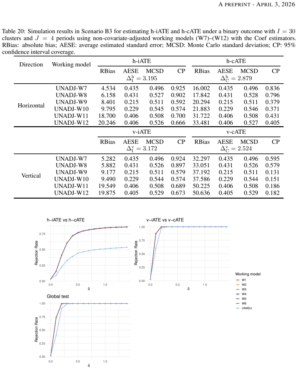
- Simulations with continuous and binary outcomes show that raw treatment-effect coefficients from standard GEE, LMM, and GLMM working models can be badly biased for cluster-average estimands under informative sizes, while the standardized versions remain nearly unbiased with near-nominal coverage.
Reading between the lines
- Outside the paper's claims: because the estimator's validity does not depend on the working model, analysts could pre-specify one estimand and one plausible model, then report all four estimands under the same model as a sensitivity analysis without redeciding the causal question.
- A natural extension the authors do not pursue is data-adaptive estimation of $m_{zj}(\cdot)$ by flexible machine learning or cross-fitting; the efficiency result suggests such an estimator should retain consistency and approach the same semiparametric efficiency bound as sample size grows.
- The horizontal versus vertical distinction could also serve as a diagnostic for calendar-time effect heterogeneity: if vertical and horizontal estimates diverge while cluster-period sizes are stable, that divergence points toward time-varying effects rather than informative sizes alone.
- The same weighting and augmentation construction carries over to parallel-arm longitudinal and cluster-randomized crossover designs with all periods eligible, so the practical payoff of the framework extends beyond stepped-wedge trials even though the paper's formal consistency theory is developed in that setting.
Signed reviews
Editorial analysis
A structured set of objections, weighed in public.
Referee Report
Summary. The paper develops a model-robust standardization framework for stepped-wedge cluster randomized trials (SW-CRTs) with informative cluster-period sizes. It defines four causal estimands—horizontal individual-average, horizontal cluster-average, vertical individual-average, and vertical cluster-average treatment effects—under a super-population model, and proposes an augmented estimator in equation (5) that combines a working outcome regression with a randomization-based correction. The central claim is that this estimator is consistent for its target estimand for any pre-specified working model, correct or misspecified, and that the optimal working model is the conditional outcome expectation E[Y_ij(z) | X_ij, N_ij]. The paper provides consistency and optimality arguments in the Web Appendices, extensive simulations for continuous and binary outcomes with up to six working models, small-cluster extensions, an R package, and reanalyses of the TSOS and ACS-QUIK trials.
Significance. If the consistency claim is fully established, this is a practically valuable contribution: it gives trial analysts an estimand-aligned alternative to conventional GEE/LMM coefficients, whose implicit weighting can target ambiguous quantities under informative sizes. The four-estimand taxonomy is clear and connects usefully to prior work by Chen and Li (2024) and Lee et al. (2025). Strengths include the reproducible MRStdLCRT R package, the broad simulation study that evaluates misspecified working models and small numbers of clusters, and the use of a 10^7-cluster super-population to compute true estimands, which makes the finite-sample coverage checks credible. The main barrier to acceptance is that the consistency proof treats the working model as a fixed function, while the implemented procedure estimates it from the same data; this gap affects the paper's central theoretical claim.
major comments (3)
- [Web Appendix C, Eqs. (12)–(13); Section 3.2] The consistency proof treats m_zj(X_ij, N_ij) as a fixed, deterministic regression function. In the actual procedure, m_zj is replaced by fitted values from GEE, LMM, or GLMM models estimated on the same data, and the paper explicitly allows semiparametric and more flexible specifications in Section 3.2. The law-of-large-numbers argument in (12)–(13) is therefore not directly applicable to the estimator actually used, because the summands share estimated parameters and are not independent across clusters. Standard AIPW theory shows that consistency with estimated nuisance functions requires additional conditions, such as cross-fitting or uniform convergence of the fitted function to a fixed limit; these conditions are neither stated nor verified. As written, the abstract claim that the estimators are consistent 'even if the working regression model is misspecified' is not proven for the estimator implemented in the simulations and software. I recommend either (i) restricting the formal theorem to working models whose fitted values converge in probability to a fixed function and stating the required regularity conditions, which would cover the parametric GEE/LMM cases, or (ii) adding a cross-fitted version of estimator (5) and proving consistency for it.
- [Web Appendix D, Eq. (14)] The optimality argument is not sufficiently precise to support the claim that E[Y_ij(z) | X_ij, N_ij] minimizes the asymptotic variance of the augmented estimator. The derivation defines p_{1,omega} as an expected ratio but then treats it as a fixed probability in the influence function, uses h(X) both as the influence function and as an arbitrary test function in Eq. (14), and considers a single augmentation term (Z - p_1)m even though estimator (5) uses two treatment-specific functions m_{1j} and m_{0j}. Additionally, the asymptotic variance is not explicitly derived under the period-weight averaging structure with random weights omega_j. The efficiency claim is secondary to consistency, but since the paper advertises that efficiency improves as the working model approaches the truth, this argument should be made rigorous or explicitly labeled as heuristic.
- [Section 5.2, Table 3] The unadjusted estimator, which is a key benchmark, shows empirical coverage of roughly 0.925–0.935 for the horizontal estimands under Scenario C3, below the nominal 0.95 level, while the MRS estimators achieve coverage near 0.95. The paper does not comment on this undercoverage. Since the jackknife variance is used for both estimators, the authors should briefly explain why the unadjusted estimator undercovers in this setting and whether this reflects finite-sample bias in the variance estimator or a known limitation of the unadjusted estimator.
minor comments (5)
- [Tables 21 and 22] The reported global test values '626' and '651' in the TSOS and ACS-QUIK tables cannot be p-values; they should presumably be 0.626 and 0.651, and the tables should be corrected.
- [Throughout] There are several typographical errors, including 'Y ale' and 'A PRIL' in the author affiliations and header, and inconsistent spacing in phrases such as 'th e', 'an d', and 'w e'; a careful proofread is needed.
- [Section 2.1 and Eq. (5)] The notation Y_ij(z) is used both for the vector of potential outcomes and for the weighted cluster-period mean; please distinguish these, for example by using boldface for the vector and a different symbol for the mean. Also, \mu^aug_{\omega,j}(z) is sometimes written without the argument z in the text; please make the notation consistent.
- [Web Appendix C] The sentence 'If the working model is correct, ... (12) = 0' should say that the expectation of (12) is zero in the limit, since the finite-sample term is not identically zero.
- [Section 3.3] In the jackknife variance formula, the notation uses \mu_\omega(z) for the jackknife mean of the LOCO estimators, but the mean is not explicitly defined before it appears in the matrix; please define it in the displayed equation.
Circularity Check
No circularity: the augmented estimator's consistency is anchored in randomization and design weights, while self-citations are contextual and non-load-bearing.
full rationale
The central derivation is self-contained rather than circular. In equation (5), the augmented estimator decomposes into the unadjusted weighted moment estimator plus an augmentation term; Web Appendix C then shows that, for any fixed working function m_zj, the augmentation term converges to a difference of expectations that cancels exactly under staggered randomization when the working model is misspecified, and equals the same target when the working model is correct. The estimands in Section 2 are defined from potential outcomes and pre-specified design weights before any working model is introduced, so there is no self-definitional reduction in which the estimand is defined by the estimator or vice versa. The optimal-model result in Web Appendix D is a standard influence-function projection argument from semiparametric theory, not an ansatz imported by citation. The paper's references to Li et al. (2025) and B. Wang et al. (2024) are self-citations, but they are used for context, comparison, or as motivation; the consistency proof in Web Appendix C does not rely on them. One genuine caveat is that the proof treats m_zj as a fixed function, whereas the procedure fits m_zj on the same data; standard AIPW theory would require extra conditions, such as cross-fitting or rate conditions, for estimated misspecified nuisances. That is a proof-hardening and correctness concern, not a circularity, because the randomization-based cancellation and the target estimand are defined independently of the fitted working model, and the simulations validate the claim against an external super-population of 10^7 clusters.
Assumptions & free parameters
free parameters (3)
- Simulation scenario parameters =
C1-C3, B1-B3: coefficients like 1 + sin(X_1) + exp(-X_2), treatment mean 8.395-8.821 in C3
- Working model specifications =
W1-W6 continuous, W7-W12 binary: period effects, treatment, covariate, size main effects
- Jackknife t degrees of freedom I-1 =
I-1
assumptions (4)
- domain assumption Super-population of clusters with I going to infinity
- domain assumption Staggered randomization: Z_ij independent of potential outcomes given baseline covariates and N_ij
- domain assumption SUTVA and no anticipation, no exposure-time treatment effect heterogeneity
- domain assumption Treatment effect contrast f(a,b) predefined
invented entities (1)
-
Four estimands: h-iATE, h-cATE, v-iATE, v-cATE
independent evidence
Cite this review
Pith. "Pith review of Model-robust standardization in stepped wedge cluster randomized trials." pith.science (2026). https://pith.science/paper/WRXSYIVU
@misc{pith2026250717190,
  author       = {Pith},
  title        = {Pith review of: Model-robust standardization in stepped wedge cluster randomized trials},
  year         = {2026},
  howpublished = {\url{https://pith.science/paper/WRXSYIVU}},
  note         = {Machine review of arXiv:2507.17190}
}
read the original abstract
Stepped-wedge cluster-randomized trials (SW-CRTs) are widely used in healthcare and implementation science, enabling all clusters to receive the intervention through a staggered rollout. Traditional model-based methods, including generalized estimating equations and mixed models, yield estimates that depend on implicit weighting schemes and parametric assumptions, and therefore may target ambiguous estimands under model misspecification. In this article, we propose a model-robust standardization framework for SW-CRTs that generalizes existing methods from parallel-arm CRTs to address informative sizes. We define causal estimands including horizontal-individual, horizontal-cluster, vertical-individual, and vertical-cluster average treatment effects under a super population framework and introduce a simple procedure that standardizes parametric and semiparametric working models for estimand-aligned analysis. For any specified working model, the resulting estimators remain consistent for their target estimands even if the working regression model is misspecified; moreover, their efficiency improves as the working model more closely approximates the true data-generating process. We evaluate the finite-sample properties of our proposed estimators through extensive simulations. Finally, we illustrate the application of our methods through reanalyses of two real-world SW-CRTs.
Figures


Figures from the paper (4 more)


Reference graph
Works this paper leans on
-
[1]
B., van der Laan, M., A yieko, J., Kamya, M., Chamie, G., Schwab, J., Havlir, D
Balzer, L. B., van der Laan, M., A yieko, J., Kamya, M., Chamie, G., Schwab, J., Havlir, D. V ., & Petersen, M. L. (2023). Two-stage tmle to reduce bias and improve efficiency in clust er randomized trials. Biostatistics, 24(2), 502–
work page 2023
-
[2]
have shown that the residual error ǫijk contributes a heteroskedastic error term with variance σ2 ǫ/Nij. However, a convenient modeling practice is to continue ass uming γ∗ ij ∼ N (0,σ 2 γ∗ ), so that standard model fitting routine for linear mixed mode ls can be used. In fact, even if such a cluster-period-level linear mixed model potentially misspecifies ...
work page 2022
-
[4]
28 A PREPRINT - A PRIL 3, 2026 A modified degree of freedom, proposed by Barnard and Rubin (1
( 1 + M M + 1 V ω(z) Bω(z) )2 . 28 A PREPRINT - A PRIL 3, 2026 A modified degree of freedom, proposed by Barnard and Rubin (1
work page 2026
-
[5]
(EMA/CHMP/ICH/436221/2017). Gasparini, A., Crowther, M. J., Hoogendijk, E. O., Li, F., & H arhay, M. O. (2025). Analysis of cohort stepped wedge cluster-randomized trials with nonignorable dropout via joint modeling. Statistics in Medicine, 44(5), e10347. Girling, A. J., & Hemming, K. (2016). Statistical efficiency and optimal design for stepped cluster st...
work page Pith review arXiv 2025
-
[6]
B Proof of the consistency of nonparametric estimators In this section, we provide proof of the consistency of ˆµunadj ω (z). By the law of large numbers, and under the assumption of SUTV A and randomization, as I → ∞, 1 I I∑ i=1 ωijI(Zij =z)Y ij p → E [ ωijI(Zij =z)Y ij ] , and 1 I I∑ i=1 ωijI(Zij =z) p → E [ωijI(Zij =z)]. Hence, by the continuous mappin...
work page 2006
-
[7]
A similar result holds for Z = 0
(14) Sincep1,ω is bounded away from zero almost surely and E{Y (1) |Z = 1, X,N } −m1(X,N ) is a function of X,N , the expectation in (14) can only be zero for all h(X) if and only if E{Y (1) |Z = 1, X,N } =m1(X,N ). A similar result holds for Z = 0 . Therefore, for each period j, the optimal augmentation function that minimizes the asymptotic variance of ...
work page 2026
-
[8]
This leads to µzj (X ij,N ij) = µzj for anyj = 2...,J − 1 andi = 1,...,I . F Specifying the working outcome regression model with clus ter-period means F .1 Linear mixed model with cluster-period-level means An alternative modeling strategy specifies a linear mixed-e ffects model directly for the cluster-period mean outcome Y ij, aggregated from the indivi...
work page 2026
-
[9]
is correlated with the horizontally aggregated cluster-s pecific treatment effect. Rejection of this null hypothesis suggests that different cluster sizes could mar ginally associate with different treatment effects, imply ing that estimands that treat individuals and clusters differe ntly may not agree due to underlying cluster size heterogene ity. The va...
work page 2026
Show all 20 references
-
[10]
In the special case where the expected cluster-period sizes do not vary across roll-out periods, thus, E { Nij ∑ J−1 s=2 Nis } = 1 J−2 for allj ∈ {2,...J − 1} the above test is algebraically equivalent J−1∑ j=2 Cov ( Nij ∑ J−1 s=2 Nis , ∑ Nij k=1{Yijk (1) −Yijk (0)} Nij ) = 0,...
2026
-
[11]
This representation implies a test for informative period size (or, equivalently, informative expected cluster-period size over calendar time)
This is equivalent to Covj E(Nij), E [ ∑ Nij k=1{Yijk (1) −Yijk (0)} ] E(Nij) = 0, where Covj(·, ·) denotes covariance across periodsj = 2,...,J −1 under the uniform distribution. This representation implies a test for informative period size (or, equivalently, info...
2025
-
[12]
both ar ms present
39 A PREPRINT - A PRIL 3, 2026 Table 8: Simulation results in Scenario C2 for estimating fo ur estimands under a continuous outcome with I = 30 clusters and J = 6 periods using non-covariate-adjusted working models (W1) -(W6) with the Coef estimators. RBias (%): absolute relat...
2025
-
[13]
The empirica l rejection rates for these tests are reported
1000 Monte Carlo iterations were conducted. The empirica l rejection rates for these tests are reported. Figure 3 summarizes the empirical rejection rates of the thr ee tests across increasing values of δ for continuous out- comes, evaluated under a range of working models. Th...
2024
-
[14]
are known by design and typically satisfy ej ∧ (1 −ej) > 0 for all j, implying that all periods j = 1,...,J are eligible in the definitions of µω(z) and τω, in contrast to SW-CRTs where periods with ej ∈ { 0, 1} at j = 1 and j = J are excluded. Figures 5 and 6 provide schematic...
2025
-
[15]
= 1 /2 for all j = 1,...,J ). As a result, all periods contributes in the definition of th e 52 A PREPRINT - A PRIL 3, 2026 Table 22: Informative cluster size test p-values for the ACS-QUIK trial under working models (W7) thr ough (W12) and unadjusted estimator (UNAJD), For eac...
2026
-
[17]
White cells in periods 1-5 indicate control cluster-periods and colored cells in periods 1-5 indicate intervention cluster-periods
A schematic illustration of different treatment effect defi nitions in a hypothetical two-arm parallel CRT with 8 cluste rs and 5 periods. White cells in periods 1-5 indicate control cluster-periods and colored cells in periods 1-5 indicate intervention cluster-periods. (a) Hor...
2026
-
[18]
cluster", period =
A schematic illustration of different treatment effect defi nitions in a hypothetical multiple-period cross-over CRT w ith 8 clusters and 5 periods. White cells in periods 1-5 indic ate control cluster-periods and colored cells in periods 1-5 indicate intervention cluster-perio...
2026
-
[23]
53 A PREPRINT - A PRIL 3, 2026 Cluster 1 Cluster 2 Cluster 3 Cluster 4 Cluster 5 Cluster 6 Cluster 7 Cluster 8 Period 1 Period 2 Period 3 Period 4 Period 5 (a) Horizontal individual-average treatment effect e1= 1 / 2 e 2= 1 / 2 e 3= 1 / 2 e 4= 1 / 2 e 5= 1 / 2 Patient-level ca...
2026
-
[29]
To define treatment effects for the implemented intervention ( see Figure 7), we allow an implementation phase whose duration may vary across clusters
Stepped-wedge edge pattern: YES (first period 1 all control ; last period 6 all treatment) ICS hypothesis test (linear-contrast F test) ------------------------------------------------------------------------ method_type df1 df2 F p_value 1 unadjusted 3 29 13.14064 1.3e-05 2 a...
-
[30]
The dashed columns indicate the baseline and final rollout periods, which are ex cluded from the estimand definition
Cluster 1 Cluster 2 Cluster 3 Cluster 4 Cluster 5 Cluster 6 Cluster 7 Cluster 8 Period 1 Period 2 Period 3 Period 4 Period 5 Period 6 Period 7 Treatment Control Implementation period baseline/final rollout e1= 0 e 2= 0 e 3= 0 e 4= 1 / 4 e 5= 1 / 2 e 6= 3 / 4 e 7= 1 Figure 7: Il...
2026
-
[517]
B., Zheng, W ., van der Laan, M
Balzer, L. B., Zheng, W ., van der Laan, M. J., & Petersen, M. L. (2019). A new approach to hierarchical data analysis: Targeted maximum likelihood estimation for the causal effe ct of a cluster-level exposure. Statistical Methods in Medical Research, 28(6), 1761–1780. Barnard...
2019
Reviewed August 6, 2026 · model on record in the stance chip above.
Discussion (0). Continue with ORCID to comment.