Stationary quasi-periodic pulsations in 20-second cadence TESS flares

Aadish Joshi; Dario J. Fritzewski; Daye Lim; Tom Van Doorsselaere

REVIEW 3 major objections 6 minor 1 cited by

Stationary quasi-periodic pulsations in 20-second cadence TESS flares

T0 review · 3 major / 6 minor · reviewed 2026-08-06 · deepseek-v4-flash

Challenge this review Re-run · record.json Download PDF Read on arXiv ↗ Review JSON

Pith's one-line read TESS data show stellar flare pulsations scale with flare duration, mirroring the Sun.

desk verdict A genuinely useful short-period QPP catalog, but the P–tau scaling law is not established; the branch is selected post hoc and the detection window itself can create the trend. read the letter →

arxiv 2506.22131 v1 pith:WUBA35IC submitted 2025-06-27 astro-ph.SR

Aadish Joshi , Tom Van Doorsselaere , Daye Lim , Dario J. Fritzewski This is my paper · ORCID

classification astro-ph.SR

keywords quasi-periodicpulsationsstellarflaresTESS20-secondcadenceAFINOARIMAflaredetectionQPPperiod–durationscalingsolar–stellaranalogy

verification ladder T0 review T1 audit T2 compute T3 formal

The pith

A machine-rendered reading of the paper's core claim, the machinery that carries it, and where it could break.

The reading

Using TESS 20-second cadence data from sectors 27–80, this study identifies 3878 flares on 1285 stars and, within 61 of those flares on 57 stars, quasi-periodic pulsations (QPPs) with periods of 42–193 seconds — a short-period regime that earlier Kepler- and TESS-based stellar surveys largely missed. The central claim is that a branch of these QPPs follows a power-law relation between oscillation period and flare duration, $P \propto \tau_{\mathrm{flare}}^{0.33 \pm 0.08}$, meaning longer-duration flares host longer-period pulsations. The authors argue that this mirrors the scaling seen in solar-flare QPPs, supporting the idea that stellar and solar QPPs share a common physical mechanism. If correct, the result makes QPP period a usable diagnostic of flare size and opens a route to seismic probing of stellar flare loops.

What carries the argument

The argument is carried by AFINO (Automated Flare Inference of Oscillations), a Fourier-domain model-comparison test that fits three models to a flare's power spectrum — a single power law, a power law with a Gaussian bump, and a broken power law — and requires a Bayesian information criterion difference of $\Delta\mathrm{BIC} > 10$ to accept the bump model. Because AFINO assumes oscillations whose amplitude and period stay roughly constant over the window, the detected QPPs are 'stationary' by construction, and short-period oscillations are favored. Flare candidates come from an ARIMA residual search that flags excursions above $3\sigma$ lasting at least eight 20-second points and validates them with fast-rise/exponential-decay shape checks. The branch correlation is produced by K-means clustering in the period–duration plane followed by Pearson and Spearman tests and a Bayesian linear regression in log–log space.

What would settle it

Run an injection-recovery experiment: embed synthetic QPPs with known periods and randomly chosen flare durations into real TESS 20-second light curves, run the same ARIMA+AFINO+K-means pipeline, and check whether a $P \propto \tau^{0.33}$ branch emerges when no true period–duration correlation exists. If it does, the observed branch is a selection effect; if not, the correlation is supported.

Watch

Extended reading notes

Core claim

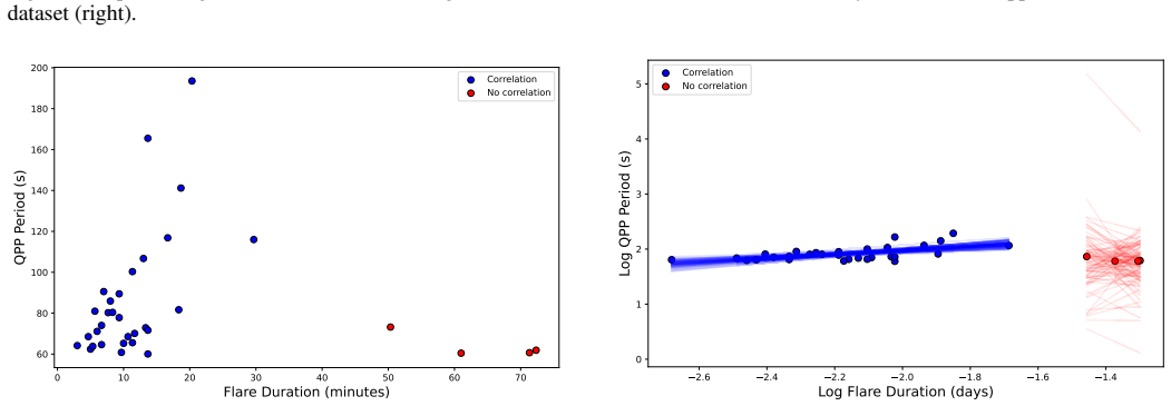
On the paper's own terms, the central discovery is that short-period stellar QPPs can be surveyed statistically in 20-second TESS observations, and that the recovered period–duration diagram contains a distinct branch — selected after visual inspection and isolated with K-means clustering — in which the QPP period grows with flare duration. For that branch the paper reports a Bayesian linear fit in log–log space of $\log P = (0.33 \pm 0.08)\log\tau_{\mathrm{flare}} - (2.59 \pm 0.17)$, i.e. $P \propto \tau_{\mathrm{flare}}^{0.33 \pm 0.08}$, with Pearson $r = 0.69$ ($p < 0.0001$) and Spearman $\rho = 0.42$ ($p = 0.011$). Restricting the analysis to QPPs with periods above 60 seconds leaves 34 events and reproduces the trend with slope $0.34 \pm 0.10$. The authors interpret the similarity of this slope to the solar-flare scaling reported in earlier work as evidence that stellar and solar QPPs are governed by analogous processes, while cautioning that the correlation appears for a branch rather than the full sample.

Load-bearing premise

The central claim assumes that the branch picked out visually and by K-means is a real physical subgroup rather than a chance arrangement, and that the period–duration trend is not a detection bias in which short flares naturally yield short periods because they contain only a few oscillation cycles.

Editorial extensions

If this is right

If the scaling is real, future 20-second TESS surveys should find that longer flares systematically host longer-period QPPs, making QPP period a predictor of flare duration.
The 42–193 second period range becomes accessible to routine optical stellar-flare studies, while surveys at 2-minute cadence are expected to miss most of these events.
The solar-like slope supports treating stellar and solar QPPs as the same phenomenon, which would extend solar flare-loop seismology to other stars.
The 61-event catalog offers a benchmark for comparing QPP detection methods, since AFINO is conservative and detects different events than wavelet- or network-based searches.
The repeated ~60-second period in two flares of one B-type subdwarf points to a stable oscillator worth targeted follow-up.

Reading between the lines

Editorial extensions of the paper, not claims the author makes directly.

The slope should be reproducible in later TESS sectors; applying the same ARIMA+AFINO pipeline to untapped sectors provides a genuine out-of-sample test of the branch.
If the scaling is physical, higher-cadence observations such as 2-second data should reveal the same branch extending below the 40-second Nyquist limit of this survey.
The two ~60-second QPPs on the B-type subdwarf motivate radial-velocity monitoring to distinguish an intrinsic oscillator from a companion-driven signal.
A natural extension the paper implies but does not perform is to inject synthetic QPPs with known periods and durations into real TESS light curves to map the detection efficiency and quantify selection effects.

Share X Bluesky LinkedIn Reddit HN

Editorial analysis

A structured set of objections, weighed in public.

Desk editor's note, referee report, and a circularity audit.

Desk Editor's Note

read the letter

Let me cut to the chase. This is a useful paper for the catalog it ships: 61 QPPs with periods 42–193 s in 20-s TESS data is a real step beyond the 9 and 17 QPPs in the earlier TESS samples. The flare detection pipeline is standard (ARIMA + thresholding), but the authors are honest about its biases — the 4-hour cut, the 160-s minimum flare duration, the low occurrence rate. The QPP detection uses AFINO, a well-tested method. The paper also reports null correlations between QPP period and stellar parameters, which is a useful negative result. I trust the catalog.

Where I part ways with the authors is the headline scaling law. The full sample shows no period–duration correlation (r=-0.042, p=0.767). The positive relation, P ∝ τ^0.33, only appears after the authors visually identify a branch in the P–τ plane and isolate it with K-means. That selection step is not folded into the significance. Under a null model, the same recipe (K-means + pick the steepest adjacent clusters) will produce a positive slope. The stress-test note is right about this.

There is also a second, independent selection effect the paper does not address: AFINO searches periods between 40 s (Nyquist) and 300 s, and a short flare simply does not have enough cycles for a long period to be detected. So even if P and τ were physically independent, the detected subset will show P increasing with τ. The robustness check that drops QPPs below 60 s repeats the same branch-selection procedure and therefore does not break the circularity. The authors themselves caution against overinterpreting the scaling, which I appreciate, but the caution is in the conclusions, not in the method.

So my verdict: the catalog is sound and worth publishing; the scaling-law claim should be clearly labeled as tentative or removed from the abstract. The comparison to solar flare scaling (Hayes et al. 2020, slope 0.67) is premature when the stellar slope 0.33 comes from a post hoc subset plus a detection bias.

Who should read this? Anyone working on stellar flare QPPs, especially the short-period regime. The catalog alone makes it worth referee time. This paper should go to peer review; a good referee will ask for a simulation-based null test of the branch selection and a correction for the detectability window. But it deserves that attention.

Referee Report

3 major / 6 minor

Summary. This paper analyzes 20-second cadence TESS light curves from sectors 27 to 80. It uses an ARIMA-based automated flare detector to report 3878 flares on 1285 stars and then applies the AFINO Fourier model-comparison method to identify 61 quasi-periodic pulsations in 57 stars, with periods between 42 and 193 seconds. The paper's central quantitative claim is a positive scaling between QPP period and flare duration, P ∝ τ^(0.33±0.08), found in a visually identified branch of the period-duration diagram and interpreted as analogous to solar-flare QPP scaling.

Significance. If validated, the claimed period-duration scaling would connect short-period stellar QPPs to the well-studied solar-flare QPP phenomenology and would provide a new observational constraint on QPP mechanisms. The catalog of 61 short-period stellar QPPs is itself a useful addition to the literature, and the paper is transparent about several limitations, including the 4-hour flare-duration cutoff and AFINO's conservative detection behavior. The availability of the detection tables in a public repository is a strength. However, the headline scaling relation is currently supported only by a post hoc selected subset of the data, while the full sample shows no correlation; the statistical demonstration therefore does not yet match the strength of the astrophysical claim.

major comments (3)

[4.2, Fig. 7(b), Fig. 9, Eq. (15)-(16)] The scaling law in Eqs. (15)-(16) is derived from a branch that the authors identify 'on visual inspection' and then isolate with K-means clustering on the same two variables (log P and log τ_flare) that are later regressed. The full sample shows no correlation (r = -0.042, p = 0.767), so the positive result exists only after selection. The p-values quoted for the branch (Spearman p = 0.0112, Pearson p = 0.0000) do not include the selection step, and under a null model with no physical P-τ relation the same 'visual branch plus K-means' recipe will still produce positive slopes. Please supply a pre-specified selection rule, a simulation-based null that includes the clustering step, or an out-of-sample validation before Eq. (16) can be taken as an astrophysical scaling law.
[4.1 and 4.2] AFINO's search is restricted to periods between 40 s (Nyquist) and 300 s and requires several resolved cycles inside the flare window. This creates a detection selection effect: short flares can only contain short-period oscillations, so even if P and τ_flare are independent, the detected subset will show P increasing with τ_flare. The period cut at 60 s and the K=2 re-clustering leading to Eq. (18) do not remove this effect, because the same branch-selection recipe is applied and the search-window constraint is unchanged. Please quantify the expected null trend by injecting synthetic oscillations with known periods into the actual flare duration distribution and running the full AFINO plus clustering pipeline.
[4.2, K-means procedure] The choice K=4 is asserted as 'optimal' without a quantitative criterion, and clusters 1-2 and 3-4 are grouped after inspecting the slopes; the reported Spearman and Pearson p-values are not corrected for this model selection. The stability of the grouping should be assessed (e.g., silhouette or gap statistic, bootstrap resampling), and the two-branch regression should be reported together with the full-sample regression so that the sensitivity of Eq. (16) to the cluster definition is visible to the reader.

minor comments (6)

[Eq. (15) vs Eq. (18)] The intercept in Eq. (15) is printed with a minus sign (-2.59), while Eq. (18) has +2.67 and the plotted range in Fig. 9 requires a positive intercept when τ_flare is in days; please correct the sign in Eq. (15) or state the units explicitly.
[4.1] The sentence 'we restricted the frequency fp to be ≤ 300 s' should read 'period' rather than 'frequency' and the units should be seconds; similarly, 'below the Nyquist frequency of 0.025 Hz or equivalently 40 s' should be phrased as 'periods shorter than 40 s' for clarity.
[4.2] The Pearson p-value is reported as 0.0000; this should be reported as p < 0.0001.
[5 and 4.2] The statement that the stellar slope 0.33 is similar to the solar slope 0.67 (Hayes et al. 2020) is not supported by overlap of the quoted values; please qualify this comparison or provide a quantitative test of similarity.
[3.1.2 and 4.2] The 4-hour duration cut is acknowledged to risk rejecting real megaflares; please state how many candidate flares are removed by this cut and whether any of the 61 QPP detections are near the cut, since this affects the interpretation of the duration distribution.
[Data availability] The data availability statement points to a GitHub repository, but no version or DOI is given; archiving the exact tables and pipeline version would improve reproducibility.

Circularity Check

2 steps flagged · score 6.0 of 10

The headline period–duration scaling (Eq. 16) is a regression on a branch that was selected because it visually shows that same correlation; the robustness check repeats the same circular selection.

self definitional [Sect. 4.2, Fig. 7(b)/Fig. 9, Eqs. (15)-(16)]
"On visual inspection, we find a branch of QPPs showing a linear correlation as highlighted in Fig. 7 (b) and in Fig 9. To separate the branch of QPPs for the analysis from the rest of the data points, K-means clustering was applied. We find that the optimal number of clusters is K = 4, where clusters 1 and 2 included the branch showing a visual correlation and clusters 3 and 4 included the rest of the data points."

The 'branch' is defined as the set of points that visually show a linear correlation in the log P versus log flare-duration plane, and K-means then isolates that same set using the same two variables that are later regressed. The Bayesian fit reported as Eq. (15)-(16) simply quantifies the visual correlation that was used to define the branch. The full-sample correlation is null (r = -0.042, p = 0.767), so the positive result exists only inside the post-hoc selected subset, with no correction for the selection step.
fitted input called prediction [Sect. 4.2, Eqs. (18)-(19)]
"After applying similar steps as the original dataset however this time with K=2 clustering, we found the Spearman and Pearson correlation coefficient of 0.52 (p-value: 0.0034) and 0.60 (p-value:0.0005) respectively for the branch showing a correlation. This results in the following scaling relationship: log P = (0.34±0.10) logτflare + (2.67±0.21)"

This robustness check repeats the same selection recipe: after excluding short-period QPPs, the remaining points are clustered in the period-duration plane and the slope is fitted to the branch 'showing a correlation' that is again identified from the visual trend. The fitted slope (0.34±0.10) is therefore not an independent confirmation of Eq. (16); it is the same quantity re-fitted to a similarly selected subset, so it cannot break the original circularity.

full rationale

The paper is largely self-contained for its catalog: AFINO is an external, published method; the 61 QPP detections and the null correlations with temperature, energy, ED, and rotation are independent empirical content. The circularity is concentrated in the headline scaling claim. The branch in Fig. 7(b)/Fig. 9 is introduced as 'a branch of QPPs showing a linear correlation' and then isolated by K-means clustering on the same log P-log tau plane; Eq. (16) is the regression of that selected branch. Because the full sample shows no period-duration correlation, the positive result is produced by the selection rather than by an independent population. The paper is transparent about the null full-sample result and explicitly cautions that the scaling holds only for a branch, which prevents a higher score; the AFINO window and finite-cycle detection effects are additional selection biases but are not themselves circular steps in the equations.

Assumptions & free parameters 10 free parameters · 6 assumptions · 0 invented entities

The central results rest on a large set of hand-chosen thresholds for flare detection (3σ, 8 points, 60% amplitude, symmetry ratio, 4h cutoff) and on the AFINO model assumptions. The scaling-law claim further depends on the K-means cluster count and on the post hoc branch definition. No new physical entities are introduced.

free parameters (10)

QPP period-duration power-law exponent = 0.33 ± 0.08
Fitted to the K-means selected branch using Bayesian linear regression in log-log space (Sect. 4.2, Eq. 16). This is the central quantitative result.
K-means cluster count K = 4 (and 2 in the P > 60 s robustness test)
Chosen as 'optimal' after visual inspection of the scatter plot to separate the branch that appears to correlate from the rest (Sect. 4.2).
Residual detection threshold = 3σ
Candidates are flagged when residuals exceed three times the standard deviation (Sect. 3.1.2).
Minimum flare length = 8 consecutive data points (160 s)
Empirical threshold to suppress false positives; short flares are missed, which shapes the sample (Sect. 3.1.2).
Local baseline variability bound = 60% of flare amplitude
The standard deviation in the 50 points before and after the event must not exceed 60% of the flare amplitude (Sect. 3.1.2).
Symmetry ratio rejection band = 0.5 to 2.0
Events with rise/decay time ratio inside this interval are rejected as too symmetric to be flares (Sect. 3.1.2).
Maximum flare duration cut = 4 hours
Events longer than 4 hours are discarded to remove false detections; the paper concedes this can reject real megaflares (Sect. 3.1.2).
AFINO search upper period = 300 s
The pulsation search was restricted to periods at or below 300 s to target short-period QPPs (Sect. 4.1).
Flare energy power-law lower bound Xmin = 5.12e31 erg
Determined by minimizing the KS statistic for the power-law fit; influences the reported α = 1.65 but not the QPP periods (Sect. 3.4).
Robustness period cut = 60 s
QPPs with periods below 60 s are excluded in a robustness check to avoid Nyquist proximity, leaving 34 events (Sect. 4.2).

assumptions (6)

domain assumption ARIMA residuals after removing the best-fit model are white noise plus flare events
The detection pipeline treats all residual excursions above 3σ as flare candidates (Sect. 3.1.2).
domain assumption Flare light curves have a fast rise and exponential decay (FRED) shape
Used in the symmetry and shape validation of candidates (Sect. 3.1.2).
domain assumption The Fourier power spectrum of a flare is a power law, optionally with a Gaussian bump (AFINO models M0, M1, M2)
The QPP detection method depends on these models and on ΔBIC > 10 (Sect. 4.1).
domain assumption QPP oscillations are stationary (constant amplitude and period) over the analyzed window
Explicitly stated as an AFINO assumption in Sect. 4.1; non-stationary and multi-period QPPs are missed.
ad hoc to paper The K-means branch represents a real subgroup rather than a chance clustering
The scaling-law fit is applied only to the selected branch after visual inspection (Sect. 4.2).
domain assumption Flare continuum emission is a 9000 K blackbody
Used for flare energy estimates via Shibayama et al. (2013); affects energies but not the QPP periods or the scaling law.

how reviews work

0 comments

Cite this review

Pith. "Pith review of Stationary quasi-periodic pulsations in 20-second cadence TESS flares." pith.science (2026). https://pith.science/paper/WUBA35IC

@misc{pith2026250622131,
  author       = {Pith},
  title        = {Pith review of: Stationary quasi-periodic pulsations in 20-second cadence TESS flares},
  year         = {2026},
  howpublished = {\url{https://pith.science/paper/WUBA35IC}},
  note         = {Machine review of arXiv:2506.22131}
}

read the original abstract

Context. Quasi-periodic pulsations (QPPs) are an inherent feature of solar and stellar flares. However, the mechanism behind them is debated hence it is necessary to further study them to obtain a complete picture of flares and their contribution to coronal heating. Aims. We analyze 20-second cadence TESS light curves from sectors 27 to 80 to detect stellar flares and QPPs. Methods. Stellar flare detection was carried out using an automated detection routine based on autoregressive integrated moving average models. QPPs were detected using a Fourier model comparison test (AFINO). Results. We detected 3878 flares across 1285 flaring stars. Notably, 61.2% of flares had a duration of less than 10 min. 61 QPPs were detected across 57 stars significantly expanding the current stellar QPP catalog. The detected periods of the QPPs were in the range of 42 to 193 seconds. In the diagram showing QPP periods against the flare duration a branch emerges. It shows a positive correlation with the flare duration, meaning longer duration flares host longer period QPPs. Conclusion. Our study detected short-period and sub-minute QPPs in stellar flares that have rarely been explored in other works. We find similar scaling laws between solar and stellar QPPs which indicates that QPPs in stellar flares might be analogous to the ones in solar flares as both show evidence of scaling with flare duration.

Figures

Figures reproduced from arXiv: 2506.22131 by the authors.

**Figure 2.** Top left: A simulated flare generated using the template from [PITH_FULL_IMAGE:figures/full_fig_p004_2.png] view at source ↗

**Figure 3.** Distribution of flare energy (left) and the cumulative flare frequency distribution with a power-law fit (right). The blue line [PITH_FULL_IMAGE:figures/full_fig_p005_3.png] view at source ↗

Figures from the paper (7 more)

**Figure 4.** Figure 4: Distribution of equivalent duration (left) and the cumulative frequency distribution with a power-law fit (right). The power [PITH_FULL_IMAGE:figures/full_fig_p005_4.png]

**Figure 5.** Figure 5: Example of a flare with a flat-top morphology (left) and a complex multi-peak structure (right). Such flares are harder to [PITH_FULL_IMAGE:figures/full_fig_p007_5.png]

**Figure 6.** Figure 6: Example of AFINO models applied to a stellar flare detected in TIC 33878971 (top panel) and TIC 303443210 (bottom [PITH_FULL_IMAGE:figures/full_fig_p009_6.png]

**Figure 7.** Figure 7: QPP periods with associated errors against various parameters: (a) Stellar e [PITH_FULL_IMAGE:figures/full_fig_p010_7.png]

**Figure 8.** Figure 8: Histogram of QPP periods detected in our sample. The [PITH_FULL_IMAGE:figures/full_fig_p011_8.png]

**Figure 9.** Figure 9: QPP periods against flare duration showing a visual correlation in blue (left) with the Bayesian linear fit applied to the same [PITH_FULL_IMAGE:figures/full_fig_p012_9.png]

**Figure 10.** Figure 10: QPP periods above 60 seconds against flare duration showing a visual correlation in blue (left) with the Bayesian linear fit [PITH_FULL_IMAGE:figures/full_fig_p012_10.png]

Discussion (0). Continue with ORCID to comment.

Forward citations

Cited by 1 Pith paper

Reviewed papers in the Pith corpus that reference this work. Sorted by Pith novelty score. Full citation record

The Study of Quasi-Periodic Pulsations in Solar and Stellar Flares with SKA
astro-ph.SR 2026-07 accept novelty 3.0 of 10

SKA’s radio imaging spectroscopy and polarisation will enable decisive tests of QPP mechanisms in solar and stellar flares, including weak events and solar–stellar comparisons.

Reference graph

Works this paper leans on

61 extracted references · 42 canonical work pages · cited by 1 Pith paper

[1]

M., Mathioudakis, M., Van Doorsselaere, T., & Kowalski, A

Anfinogentov, S., Nakariakov, V . M., Mathioudakis, M., Van Doorsselaere, T., & Kowalski, A. F. 2013, ApJ, 773, 156 Astropy Collaboration, Robitaille, T. P., Tollerud, E. J., et al. 2013, A&A, 558, A33

work page 2013
[2]

A., Broomhall, A

Balona, L. A., Broomhall, A. M., Kosovichev, A., et al. 2015, MNRAS, 450, 956

work page 2015
[3]

A., Kolotkov, D

Belov, S. A., Kolotkov, D. Y ., Nakariakov, V . M., & Broomhall, A.-M. 2024, ApJS, 274, 31

work page 2024
[4]

J., Koch, D., Basri, G., et al

Borucki, W. J., Koch, D., Basri, G., et al. 2010, Science, 327, 977

2010
[5]

& Jenkins, G

Box, G. & Jenkins, G. 1970, Time Series Analysis: Forecasting and Control, Holden-Day series in time series analysis and digital processing (Holden- Day)

work page 1970
[6]

Broomhall, A.-M., Davenport, J. R. A., Hayes, L. A., et al. 2019, ApJS, 244, 44

work page 2019
[7]

2024, A&A, 686, A239

Bruno, G., Pagano, I., Scandariato, G., et al. 2024, A&A, 686, A239

2024
[8]

L., Angus, R., David, T., et al

Colman, I. L., Angus, R., David, T., et al. 2024, AJ, 167, 189

2024

Show all 61 references

[9]

Davenport, J. R. A. 2016, ApJ, 829, 23

2016
[10]

Davenport, J. R. A., Hawley, S. L., Hebb, L., et al. 2014, ApJ, 797, 122

2014
[11]

Edwin, P. M. & Roberts, B. 1983, Sol. Phys., 88, 179

1983
[12]

E., Linsky, J

Gary, D. E., Linsky, J. L., & Dulk, G. A. 1982, ApJ, 263, L79

1982
[13]

Gershberg, R. E. 1972, Ap&SS, 19, 75

1972
[14]

2011, A&A, 533, A61 Günther, M

Gruber, D., Lachowicz, P., Bissaldi, E., et al. 2011, A&A, 533, A61 Günther, M. N., Zhan, Z., Seager, S., et al. 2020, AJ, 159, 60

2011
[15]

T., & Rodono, M

Haisch, B., Strong, K. T., & Rodono, M. 1991, ARA&A, 29, 275

1991
[16]

R., Millman, K

Harris, C. R., Millman, K. J., van der Walt, S. J., et al. 2020, Nature, 585, 357

2020
[17]

Hawley, S. L. & Fisher, G. H. 1992, X-Ray-heated Models of Stellar Flare At- mospheres: Theory and Comparison with Observations: Erratum

1992
[18]

A., Gallagher, P

Hayes, L. A., Gallagher, P. T., Dennis, B. R., et al. 2019, ApJ, 875, 33

2019
[19]

A., Inglis, A

Hayes, L. A., Inglis, A. R., Christe, S., Dennis, B., & Gallagher, P. T. 2020, ApJ, 895, 50

2020
[20]

Howard, W. S. & MacGregor, M. A. 2022, ApJ, 926, 204

2022
[21]

Hunter, J. D. 2007, Computing in Science & Engineering, 9, 90

2007
[22]

J., Davenport, J

Ilin, E., Schmidt, S. J., Davenport, J. R. A., & Strassmeier, K. G. 2019, A&A, 622, A133

2019
[23]

J., Poppenhäger, K., et al

Ilin, E., Schmidt, S. J., Poppenhäger, K., et al. 2021, A&A, 645, A42

2021
[24]

Inglis, A. R. & Hayes, L. A. 2024, ApJ, 971, 29

2024
[25]

R., Ireland, J., Dennis, B

Inglis, A. R., Ireland, J., Dennis, B. R., Hayes, L., & Gallagher, P. 2016, ApJ, 833, 284

2016
[26]

R., Ireland, J., & Dominique, M

Inglis, A. R., Ireland, J., & Dominique, M. 2015, ApJ, 798, 108

2015
[27]

Jackman, J. A. G., Wheatley, P. J., Acton, J. S., et al. 2021, MNRAS, 504, 3246

2021
[28]

A., Botha, G

Karampelas, K., McLaughlin, J. A., Botha, G. J. J., & Régnier, S. 2023, ApJ, 943, 131

2023
[29]

Kosovichev, A. G. & Zharkova, V . V . 2001, ApJ, 550, L105

2001
[30]

Kowalski, A. F. 2024, Living Reviews in Solar Physics, 21, 1

2024
[31]

F., Hawley, S

Kowalski, A. F., Hawley, S. L., Wisniewski, J. P., et al. 2013, ApJS, 207, 15

2013
[32]

F., Wisniewski, J

Kowalski, A. F., Wisniewski, J. P., Hawley, S. L., et al. 2019, ApJ, 871, 167

2019
[33]

2020, Solar- Terrestrial Physics, 6, 3

Kupriyanova, E., Kolotkov, D., Nakariakov, V ., & Kaufman, A. 2020, Solar- Terrestrial Physics, 6, 3

2020
[34]

D., Bagnulo, S., Fossati, L., Jordan, S., & O’Toole, S

Landstreet, J. D., Bagnulo, S., Fossati, L., Jordan, S., & O’Toole, S. J. 2012, A&A, 541, A100

2012
[35]

Lang, K. R. & Willson, R. F. 1986, ApJ, 305, 363 Lightkurve Collaboration, Cardoso, J. V . d. M., Hedges, C., et al. 2018, Lightkurve: Kepler and TESS time series analysis in Python, Astrophysics Source Code Library, record ascl:1812.013

1986
[36]

H., Williams, D

Mathioudakis, M., Seiradakis, J. H., Williams, D. R., et al. 2003, A&A, 403, 1101

2003
[37]

2010, in Proceedings of the 9th Python in Science Conference, ed

McKinney, W. 2010, in Proceedings of the 9th Python in Science Conference, ed. S. van der Walt & J. Millman, 51 – 56

2010
[38]

A., Nakariakov, V

McLaughlin, J. A., Nakariakov, V . M., Dominique, M., Jelínek, P., & Takasao, S. 2018, Space Sci. Rev., 214, 45

2018
[39]

Million, C., Kolotkov, D., & Fleming, S. W. 2021, in The 20.5th Cambridge Workshop on Cool Stars, Stellar Systems, and the Sun (CS20.5), Cambridge Workshop on Cool Stars, Stellar Systems, and the Sun, 272

2021
[40]

J., van Driel-Gesztelyi, L., & Baker, D

Murray, M. J., van Driel-Gesztelyi, L., & Baker, D. 2009, A&A, 494, 329

2009
[41]

Pandey, J. C. & Srivastava, A. K. 2009, ApJ, 697, L153

2009
[42]

2024, arXiv e-prints, arXiv:2412.07580

Panferov, A., Beskin, G., Karpov, S., & Maryeva, O. 2024, arXiv e-prints, arXiv:2412.07580

2024 arXiv
[43]

Pecaut, M. J. & Mamajek, E. E. 2013, ApJS, 208, 9

2013
[44]

2022, ApJ, 935, 143

Pietras, M., Falewicz, R., Siarkowski, M., Bicz, K., & Pre ´s, P. 2022, ApJ, 935, 143

2022
[45]

E., Armstrong, D

Pugh, C. E., Armstrong, D. J., Nakariakov, V . M., & Broomhall, A. M. 2016, MNRAS, 459, 3659

2016
[46]

E., Broomhall, A

Pugh, C. E., Broomhall, A. M., & Nakariakov, V . M. 2019, A&A, 624, A65

2019
[47]

Myagkova, I. N. 2017, A&A, 608, A101

2017
[48]

G., & Doyle, L

Ramsay, G., Kolotkov, D., Doyle, J. G., & Doyle, L. 2021, Sol. Phys., 296, 162

2021
[49]

R., Winn, J

Ricker, G. R., Winn, J. N., Vanderspek, R., et al. 2014, in Society of Photo- Optical Instrumentation Engineers (SPIE) Conference Series, V ol. 9143, Space Telescopes and Instrumentation 2014: Optical, Infrared, and Millime- ter Wave, ed. J. Oschmann, Jacobus M., M. Clampin, G...

2014
[50]

R., Winn, J

Ricker, G. R., Winn, J. N., Vanderspek, R., et al. 2015, Journal of Astronomical

2015
[51]

A., Bergeron, P., Koester, D., & Liebert, J

Saffer, R. A., Bergeron, P., Koester, D., & Liebert, J. 1994, ApJ, 432, 351

1994
[52]

V ., & Fonnesbeck, C

Salvatier, J., Wiecki, T. V ., & Fonnesbeck, C. 2016, PeerJ Computer Science, 2, e55

2016
[53]

2013, ApJS, 209, 5

Shibayama, T., Maehara, H., Notsu, S., et al. 2013, ApJS, 209, 5

2013
[54]

Smith, T. G. et al. 2017, pmdarima: ARIMA estimators for Python, [Online; accessed <today>]

2017
[55]

F., & Wang, F

Tu, Z.-L., Yang, M., Wang, H. F., & Wang, F. Y . 2021, ApJS, 253, 35 Van Doorsselaere, T., Kupriyanova, E. G., & Yuan, D. 2016, Sol. Phys., 291, 3143 Van Doorsselaere, T., Shariati, H., & Debosscher, J. 2017, ApJS, 232, 26

2021
[56]

E., et al

Virtanen, P., Gommers, R., Oliphant, T. E., et al. 2020, Nature Methods, 17, 261

2020
[57]

Y ., Wheatley, J., Browne, S

Welsh, B. Y ., Wheatley, J., Browne, S. E., et al. 2006, A&A, 458, 921

2006
[58]

& Liu, J

Yang, H. & Liu, J. 2019, ApJS, 241, 29

2019
[59]

V ., Kislyakov, A

Zaitsev, V . V ., Kislyakov, A. G., Stepanov, A. V ., Kliem, B., & Furst, E. 2004, Astronomy Letters, 30, 319

2004
[60]

L., & Misra, P

Zhang, L., Yang, Z., Su, T., Han, X. L., & Misra, P. 2024, A&A, 689, A103

2024
[61]

V ., McLaughlin, J

Zimovets, I. V ., McLaughlin, J. A., Srivastava, A. K., et al. 2021, Space Sci. Rev., 217, 66 Article number, page 13

2021

Pith tools

Reviewed August 6, 2026 · model on record in the stance chip above.

[1] [1]

M., Mathioudakis, M., Van Doorsselaere, T., & Kowalski, A

Anfinogentov, S., Nakariakov, V . M., Mathioudakis, M., Van Doorsselaere, T., & Kowalski, A. F. 2013, ApJ, 773, 156 Astropy Collaboration, Robitaille, T. P., Tollerud, E. J., et al. 2013, A&A, 558, A33

work page 2013

[2] [2]

A., Broomhall, A

Balona, L. A., Broomhall, A. M., Kosovichev, A., et al. 2015, MNRAS, 450, 956

work page 2015

[3] [3]

A., Kolotkov, D

Belov, S. A., Kolotkov, D. Y ., Nakariakov, V . M., & Broomhall, A.-M. 2024, ApJS, 274, 31

work page 2024

[4] [4]

J., Koch, D., Basri, G., et al

Borucki, W. J., Koch, D., Basri, G., et al. 2010, Science, 327, 977

2010

[5] [5]

& Jenkins, G

Box, G. & Jenkins, G. 1970, Time Series Analysis: Forecasting and Control, Holden-Day series in time series analysis and digital processing (Holden- Day)

work page 1970

[6] [6]

Broomhall, A.-M., Davenport, J. R. A., Hayes, L. A., et al. 2019, ApJS, 244, 44

work page 2019

[7] [7]

2024, A&A, 686, A239

Bruno, G., Pagano, I., Scandariato, G., et al. 2024, A&A, 686, A239

2024

[8] [8]

L., Angus, R., David, T., et al

Colman, I. L., Angus, R., David, T., et al. 2024, AJ, 167, 189

2024