REVIEW 3 major objections 4 minor 87 references
Risk forecasting using Long Short-Term Memory Mixture Density Networks
T0 review · 3 major / 4 minor · reviewed 2026-08-10 · deepseek-v4-flash
Pith's one-line read The paper tests whether LSTM-MDNs can compete with established Value-at-Risk models, finding them viable but not superior and dependent on large training sets and weight initialization.
desk verdict A clean, honest empirical comparison that confirms the prior result that LSTM-MDNs don't beat GARCH for 99% daily VaR, with the 3-component variant adding little; the updateding asymmetry is real but the conclusion is conservative, not inflated. read the letter →
The pith
A machine-rendered reading of the paper's core claim, the machinery that carries it, and where it could break.
The reading
What carries the argument
The central object is the LSTM mixture density network: an LSTM hidden layer that reads a sequence of daily returns and feeds a mixture-density output layer, which returns the component weights, means, and standard deviations $(\pi_k,\mu_k,\sigma_k)$ of a $K$-component Gaussian mixture for the next day's return. Two-component and three-component variants are trained by minimizing the negative log-likelihood of the mixture, with one variant adding an L2 penalty on the $\pi$'s. One-day-ahead VaR is then the empirical $\alpha$-quantile of 100,000 Monte Carlo losses drawn from the predicted mixture. The recurrent hidden state is the mechanism expected to carry information about past volatility, which is how the network accounts for volatility clustering.
What would settle it
Re-run the six evaluations with each LSTM-MDN refit every 20 trading days on all data available up to that day; if the neural networks then pass the conditional coverage test in most calm-period cases and still match GARCH in turbulent periods, the paper's conclusion that LSTM-MDNs offer only modest potential for practical use would be overturned.
Extended reading notes
Core claim
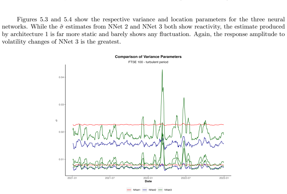
On the paper's own terms, the central claim is that LSTM-MDNs are a workable but not superior alternative to GARCH for daily 99% Value-at-Risk, with performance strongly shaped by market regime, training-set size, and random initialization. Across six backtests, the neural networks pass the conditional coverage tests in only 4 of 9 calm-period cases but in 8 of 9 turbulent-period cases, while GARCH remains the most consistently reliable single model. The LSTM mechanism does give the networks a real ability to react to short-term volatility shifts, mainly through time-varying location and variance parameters rather than through the mixture weights, and the paper is the first to test a three-component mixture in this setting. The paper also identifies two blockers to practical use: forecasts depend heavily on which random seed initializes the weights, and performance improves when the training set is large.
Load-bearing premise
The comparison treats one fixed training of each LSTM-MDN as comparable to benchmark models that are re-estimated every day on a rolling 250-day window, so the reported underperformance in calm periods could stem from this unequal updating rather than from the network itself.
Editorial extensions
If this is right
- LSTM-MDNs do not displace GARCH for daily 99% VaR on the tested indices; a simpler GARCH(1,1) with GED innovations is at least as accurate and much cheaper to run.
- The networks' strongest results appear in high-volatility periods with larger training sets, so any practical deployment should be conditioned on market regime and data availability.
- The three-component mixture is a viable addition to VaR forecasting and in some evaluations reacts to volatility shifts with the largest amplitude of the three architectures.
- The regularized two-component loss does not deliver the clear accuracy gain reported in earlier work, so its benefit is not confirmed here.
- Weight initialization is a first-order practical issue: different initial seeds can produce materially different risk forecasts.
Reading between the lines
- A fairer comparison would refit the neural networks periodically on an expanding window, as the benchmarks are refitted daily; doing so would likely change both the calm-period and turbulent-period results.
- A testable extension is to refit every 20 trading days and re-run the six backtests; if the calm-period failures disappear, the paper's 'modest potential' verdict would be a property of static training rather than of the architecture.
- Because volatility clustering is carried by $\mu$ and $\sigma$ rather than by $\pi$, a simpler recurrent model emitting a time-varying variance might capture much of the same benefit at lower cost.
- The best-of-three seed selection used in training likely paints an optimistic picture; reporting the full distribution of outcomes across seeds would show how much of the result is luck of the draw.
Editorial analysis
A structured set of objections, weighed in public.
Referee Report
Summary. The manuscript implements three Long Short-Term Memory Mixture Density Network (LSTM-MDN) variants for one-day-ahead 99% Value-at-Risk forecasting: a two-component network, a two-component network with an L2-regularized loss, and a three-component network, the last being described as new in this context. These are compared with historical simulation, the constant mean model, and GARCH(1,1) on three stock indices (FTSE 100, S&P 500, EURO STOXX 50) over two two-year evaluation windows, one calm (2017-2018) and one turbulent (2021-2022). Forecast adequacy is assessed with Kupiec's unconditional coverage test, Christoffersen's independence test, and the joint conditional coverage test, and volatility-clustering behaviour is examined through correlations between VaR forecasts and rolling realized volatility. The paper concludes that LSTM-MDNs produce adequate risk forecasts in some settings, can capture volatility clustering in a manner comparable to GARCH, but are not clearly superior to established benchmarks and are hampered by training-data requirements and sensitivity to weight initialization.
Significance. If the central comparison were conducted under a fully symmetric and reproducible protocol, the study would provide a useful independent benchmark for a recent deep-learning approach in a standard risk-management evaluation framework. The manuscript has several strengths: it uses a conventional train/validation/test split, applies well-credited backtesting tests, evaluates three architectures including a novel three-component MDN, and makes its code and data available through a repository. The correlation analysis with rolling volatility, while indirect, is a concrete attempt to measure a mechanism often discussed only qualitatively. However, the significance of the headline conclusion is substantially reduced by an asymmetric estimation protocol and by incomplete reporting of the seed-selection procedure; these issues need to be resolved before the comparative claims can be accepted.
major comments (3)
- [Section 3.2 vs. Sections 3.3.2 and 3.4; Table 5.1] The comparison of forecast accuracy is asymmetric. The benchmark models (HS, CMM, GARCH) are re-estimated daily on a rolling 250-day window (Section 3.2), whereas each LSTM-MDN is trained once on a fixed pre-evaluation set and is then used unchanged for the entire two-year evaluation period (Sections 3.3.2 and 3.4, with training-set sizes in Table 5.1). The reported differences therefore conflate model architecture with updating policy, so the abstract's claim that LSTM-MDNs are 'adequate but not superior' is not fully supported by the evidence. The manuscript itself acknowledges this in Section 5.3 ('Mitigating the data requirements could be achieved with regularly refitting the neural networks on all data which is available at time point t'), but leaves this as future work. A fair comparison requires either a refitting schedule for the neural networks or a fixed-window benchmark; without this, the central comparative conclusion remains open.
- [Section 3.3.2, 'Weight initialization'; Section 5.1.3] The best-of-three initialization procedure is not described precisely enough to support the conclusions drawn about initialization sensitivity. It is not stated whether the 'seed providing the best results on average' is selected on the validation set or on the evaluation period, and no results for the non-selected seeds or any measure of seed-to-seed variability are reported. Given that Section 5.1.3 identifies weight initialization as a key driver of model performance and unreliability, the reader cannot tell whether the presented backtests reflect a typical model or an optimistic selection. Please specify the selection metric (e.g., lowest validation loss) and report sensitivity to the three seeds for at least one index-period pair.
- [Section 5.1.2, Table 5.2] The conclusion that LSTM-MDNs capture volatility clustering 'in a comparable way as the GARCH models' is stronger than the evidence in Table 5.2 appears to justify. The reported Pearson correlations between rolling volatility (d=5) and VaR forecasts are generally lower for the neural networks than for GARCH, and some entries are negative (S&P 500 NNet1 turbulent period: -0.240; EURO STOXX 50 NNet2 calm period: -0.245), indicating a failure to track volatility in those cases. Simple correlation with rolling realized volatility is also not a direct test of clustering dynamics; it does not establish that the VaR forecasts react to volatility in a manner equivalent to GARCH. A more direct comparison of conditional-volatility responses, or a statistical test of the difference in correlations, is needed before the volatility-clustering claim can be accepted.
minor comments (4)
- [Equation (2.20)] The Kupiec POF statistic as printed contains a typographical error: the term (α̂/1)^{I(α)} should be (α̂/(1-α))^{I(α)}, since the expected violation proportion under the null is 1-α. The p-values in Tables 4.1-4.6 appear to be computed from the correct formula, so this is a presentation issue, but it should be corrected to avoid misleading readers.
- [Section 3.3.2] The text states that the networks contain 6 nodes in the LSTM layer and 10 nodes in the Dense layer, but the architecture boxes for NNet 1, NNet 2, and NNet 3 all list 'Dense-Layer [12 nodes]'. These numbers should be reconciled.
- [Chapter 4, Figures 4.1-4.6] The forecast plots do not label the benchmark-model VaR curves; adding a legend identifying V aR_HS, V aR_CMM, and V aR_GARCH alongside the NNet curves would make the visual comparisons in Section 5.1.1 much easier to verify.
- [Section 2.4 and Chapter 4] The evaluation runs six index-period combinations and several tests per model at a 5% significance level, but no multiple-testing correction is discussed. If the six evaluations are treated as independent replications this is acceptable, but the manuscript should state this explicitly rather than implicitly treating each individual p-value as decisive.
Circularity Check
No circularity: LSTM-MDN forecasts are trained on pre-evaluation data and evaluated on holdout periods against externally implemented benchmarks; the static-training versus rolling-refit asymmetry is a fairness concern, not a circularity.
full rationale
I walked the paper's derivation chain and found no step in which a claimed prediction or first-principles result is equivalent to its inputs by construction. The LSTM-MDN is trained on pre-evaluation returns using negative log-likelihood (and a regularized variant) as the loss function; one-day-ahead VaR is then produced by Monte Carlo sampling from the estimated Gaussian mixture and taking the empirical alpha-quantile (Section 3.3.3, Eq. 3.4). Neither the loss nor the sampling procedure uses the realized VaR violations or the backtest statistics as inputs, so the backtesting results are genuine holdout evaluations rather than fits renamed as predictions. The benchmark models are implemented externally (historical simulation, CMM, and GARCH); their VaR forecasts are independently re-estimated on rolling 250-day windows. The paper's central comparison therefore does not reduce to any fitted parameter or self-citation. The only notable caveat is the protocol asymmetry noted in Section 3.2 versus Section 3.4 and acknowledged in Section 5.3: benchmarks are refitted daily while each neural network is trained once and applied over the entire two-year evaluation window. This is a fairness and external-validity concern about whether the comparison disadvantages the neural networks, but it is not circularity, because the neural network forecasts remain out-of-sample predictions generated from a fixed fitted model. Citations to prior work such as Arimond et al. (2020) and Karlsson Lille and Saphir (2021) are used for architectural inspiration and for explaining conservative behaviour, not as load-bearing evidence that forces the paper's empirical results; there is no uniqueness theorem imported from the authors, no ansatz smuggled in solely through citation, and no known empirical result merely renamed under new coordinates. The paper's own limitation statements about data requirements and refitting are appropriately flagged as future work, and they support a skepticism score about comparative fairness, not a circularity score.
Assumptions & free parameters
free parameters (4)
- L2 regularization strength lambda =
0.1
- Lookback window d =
10
- LSTM and Dense layer sizes =
6 LSTM nodes, 12 Dense nodes
- Seeds for best-of-three initialization =
911, 6969, 9999
assumptions (4)
- domain assumption MDN Gaussian mixture is an adequate conditional density for daily returns
- standard math Backtest test statistics are asymptotically chi-square in samples of about 250 to 500 days
- ad hoc to paper Volatility clustering is operationalized by Pearson correlation between rolling volatility (d=5) and VaR forecasts
- domain assumption LSTM hidden state can capture dependencies beyond the d=10 input window
Cite this review
Pith. "Pith review of Risk forecasting using Long Short-Term Memory Mixture Density Networks." pith.science (2026). https://pith.science/paper/XOK7HN4L
@misc{pith2026250101278,
  author       = {Pith},
  title        = {Pith review of: Risk forecasting using Long Short-Term Memory Mixture Density Networks},
  year         = {2026},
  howpublished = {\url{https://pith.science/paper/XOK7HN4L}},
  note         = {Machine review of arXiv:2501.01278}
}
read the original abstract
This work aims to implement Long Short-Term Memory mixture density networks (LSTM-MDNs) for Value-at-Risk forecasting and compare their performance with established models (historical simulation, CMM, and GARCH) using a defined backtesting procedure. The focus was on the neural network's ability to capture volatility clustering and its real-world applicability. Three architectures were tested: a 2-component mixture density network, a regularized 2-component model (Arimond et al., 2020), and a 3-component mixture model, the latter being tested for the first time in Value-at-Risk forecasting. Backtesting was performed on three stock indices (FTSE 100, S&P 500, EURO STOXX 50) over two distinct two-year periods (2017-2018 as a calm period, 2021-2022 as turbulent). Model performance was assessed through unconditional coverage and independence assumption tests. The neural network's ability to handle volatility clustering was validated via correlation analysis and graphical evaluation. Results show limited success for the neural network approach. LSTM-MDNs performed poorly for 2017/2018 but outperformed benchmark models in 2021/2022. The LSTM mechanism allowed the neural network to capture volatility clustering similarly to GARCH models. However, several issues were identified: the need for proper model initialization and reliance on large datasets for effective learning. The findings suggest that while LSTM-MDNs provide adequate risk forecasts, further research and adjustments are necessary for stable performance.
Figures


Figures from the paper (16 more)



Reference graph
Works this paper leans on
-
[1]
Abadi, M., Agarwal, A., Barham, P., Brevdo, E., Chen, Z., Citro, C., Corrado, G. S., Davis, A., Dean, J., Devin, M., Ghemawat, S., Goodfellow, I., Harp, A., Irving, G., Isard, M., Jia, Y., Jozefowicz, R., Kaiser, L., Kudlur, M., Levenberg, J., Man\' e , D., Monga, R., Moore, S., Murray, D., Olah, C., Schuster, M., Shlens, J., Steiner, B., Sutskever, I., T...
2015
-
[2]
Alexander, C. (2005). The Present and Future of Financial Risk Management . Journal of Financial Econometrics , 3(1):3--25
2005
-
[3]
G., Bollerslev, T., Christoffersen, P
Andersen, T. G., Bollerslev, T., Christoffersen, P. F., and Diebold, F. X. (2006). Volatility and correlation forecasting. Handbook of economic forecasting , 1:777--878
2006
-
[4]
Arian, H., Moghimi, M., Tabatabaei, E., and Zamani, S. (2022). Encoded value-at-risk: A machine learning approach for portfolio risk measurement. Mathematics and Computers in Simulation , 202:500--525
2022
-
[5]
Arimond, A., Borth, D., Hoepner, A., Klawunn, M., and Weisheit, S. (2020). Neural networks and value at risk. arXiv preprint arXiv:2005.01686
work page Pith review arXiv 2020
-
[6]
Best, P. (2000). Implementing value at risk , page 10. John Wiley & Sons
2000
-
[7]
Bishop, C. M. (1994). Mixture density networks
1994
-
[8]
Bollerslev, T. (1986). Generalized autoregressive conditional heteroskedasticity. Journal of econometrics , 31(3):307--327
1986
Show all 87 references
-
[9]
Bond, P., Edmans, A., and Goldstein, I. (2012). The real effects of financial markets. Annu. Rev. Financ. Econ. , 4(1):339--360
2012
-
[10]
Brando Guillaumes, A. (2017). Mixture density networks for distribution and uncertainty estimation. Master's thesis, Universitat Polit \`e cnica de Catalunya
2017
-
[11]
Brownlee, J. (2019). A gentle introduction to the rectified linear unit (relu). https://machinelearningmastery.com/rectified-linear-activation-function-for-deep-learning-neural-networks/. visited on 2023-07-17
2019
-
[12]
Brownlee, J. (2021). How to choose an activation function for deep learning. https://machinelearningmastery.com/choose-an-activation-function-for-deep-learning/. visited on 2023-07-15
2021
-
[13]
and Chlebus, M
Buczynski, M. and Chlebus, M. (2023). Garchnet: Value-at-risk forecasting with garch models based on neural networks. Computational Economics , pages 1--31
2023
-
[14]
Y., Lo, A
Campbell, J. Y., Lo, A. W., MacKinlay, A. C., and Whitelaw, R. F. (1998). The econometrics of financial markets. Macroeconomic Dynamics , 2(4):559--562
1998
-
[15]
Campbell, S. D. (2005). A review of backtesting and backtesting procedures
2005
-
[16]
D., Teoh, E
Chen, Z., Van Khoa, L. D., Teoh, E. N., Nazir, A., Karuppiah, E. K., and Lam, K. S. (2018). Machine learning techniques for anti-money laundering (aml) solutions in suspicious transaction detection: a review. Knowledge and Information Systems , 57:245--285
2018
-
[17]
Chollet, F. et al. (2015). Keras
2015
-
[18]
B., and LeCun, Y
Choromanska, A., Henaff, M., Mathieu, M., Arous, G. B., and LeCun, Y. (2015). The loss surfaces of multilayer networks. In Artificial intelligence and statistics , pages 192--204. PMLR
2015
-
[19]
Christoffersen, P. (2008). Backtesting. Available at SSRN 2044825
2008
-
[20]
Christoffersen, P. F. (1998). Evaluating interval forecasts. International economic review , pages 841--862
1998
-
[21]
Clevert, D.-A., Unterthiner, T., and Hochreiter, S. (2015). Fast and accurate deep network learning by exponential linear units (elus). arXiv preprint arXiv:1511.07289
2015 arXiv
-
[22]
Cont, R. (2007). Volatility clustering in financial markets: empirical facts and agent-based models. In Long memory in economics , pages 289--309. Springer
2007
-
[23]
G., Vermunt, J
Dias, J. G., Vermunt, J. K., and Ramos, S. (2015). Clustering financial time series: New insights from an extended hidden markov model. European Journal of Operational Research , 243(3):852--864
2015
-
[24]
Duan, Y., Li, L., Ji, G., and Cai, Y. (2022). Vanilla feedforward neural networks as a discretization of dynamic systems. arXiv preprint arXiv:2209.10909
2022 arXiv
-
[25]
O., Martin, C
Ellefsen, K. O., Martin, C. P., and Torresen, J. (2019). How do mixture density rnns predict the future? arXiv preprint arXiv:1901.07859
2019 arXiv
-
[26]
Engle, R. F. (1982). Autoregressive conditional heteroscedasticity with estimates of the variance of united kingdom inflation. Econometrica: Journal of the econometric society , pages 987--1007
1982
-
[27]
Fausett, L. (1994). Fundamentals of neural networks: Architectures, algorithms, and applications.., new jersey, usa: Prenctice-hall
1994
-
[28]
Fons, E., Dawson, P., Zeng, X.-j., Keane, J., and Iosifidis, A. (2020). Evaluating data augmentation for financial time series classification. arXiv preprint arXiv:2010.15111
2020 arXiv
-
[29]
Glasserman, P., Heidelberger, P., and Shahabuddin, P. (2000). Efficient monte carlo methods for value-at-risk
2000
-
[30]
and Bengio, Y
Glorot, X. and Bengio, Y. (2010). Understanding the difficulty of training deep feedforward neural networks. In Proceedings of the thirteenth international conference on artificial intelligence and statistics , pages 249--256. JMLR Workshop and Conference Proceedings
2010
-
[31]
Goodfellow, I., Bengio, Y., and Courville, A. (2016). Deep learning , page 201. MIT press
2016
-
[32]
Graves, A. (2013). Generating sequences with recurrent neural networks. arXiv preprint arXiv:1308.0850
2013 arXiv
-
[33]
Gu, S., Kelly, B., and Xiu, D. (2020). Empirical asset pricing via machine learning. The Review of Financial Studies , 33(5):2223--2273
2020
-
[34]
Gupta, N. et al. (2013). Artificial neural network. Network and Complex Systems , 3(1):24--28
2013
-
[35]
Hansen, P. R. and Lunde, A. (2005). A forecast comparison of volatility models: does anything beat a garch (1, 1)? Journal of applied econometrics , 20(7):873--889
2005
-
[36]
He, K., Zhang, X., Ren, S., and Sun, J. (2015). Delving deep into rectifiers: Surpassing human-level performance on imagenet classification. In Proceedings of the IEEE international conference on computer vision , pages 1026--1034
2015
-
[37]
Hellermann, J., Qian, Q., and Shah, A. (2022). Financial time series data augmentation with generative adversarial networks and extended intertemporal return plots. arXiv preprint arXiv:2205.08924
2022 arXiv
-
[38]
Holton, G. A. (2002). History of value-at-risk
2002
-
[39]
and Raghuram, S
Kagalkar, A. and Raghuram, S. (2020). Cordic based implementation of the softmax activation function. In 2020 24th International Symposium on VLSI Design and Test (VDAT) , pages 1--4. IEEE
2020
-
[40]
Kalman, B. L. and Kwasny, S. C. (1992). Why tanh: choosing a sigmoidal function. In [Proceedings 1992] IJCNN International Joint Conference on Neural Networks , volume 4, pages 578--581. IEEE
1992
-
[41]
and Saphir, D
Karlsson Lille, W. and Saphir, D. (2021). Value at risk estimation with neural networks: A recurrent mixture density approach
2021
-
[42]
Kim, Y. (2016). Chapter 10, sequence modeling: Recurrent and recursive nets. dated Apr , 1:50
2016
-
[43]
Kingma, D. P. and Ba, J. (2014). Adam: A method for stochastic optimization. arXiv preprint arXiv:1412.6980
2014 arXiv
-
[44]
Kumar, S. K. (2017). On weight initialization in deep neural networks. arXiv preprint arXiv:1704.08863
2017 arXiv
-
[45]
Kupiec, P. H. (1995). Techniques for verifying the accuracy of risk measurement models. The Journal of Derivatives , 3(2):73--84
1995
-
[46]
Kwiatkowski, R. (2021). How to choose an activation function for deep learning. https://towardsdatascience.com/gradient-descent-algorithm-a-deep-dive-cf04e8115f21. visited on 2023-07-15
2021
-
[47]
Lu, L., Shin, Y., Su, Y., and Karniadakis, G. E. (2019). Dying relu and initialization: Theory and numerical examples. arXiv preprint arXiv:1903.06733
2019 arXiv
-
[48]
M., McCurdy, T
Maheu, J. M., McCurdy, T. H., and Song, Y. (2012). Components of bull and bear markets: bull corrections and bear rallies. Journal of Business & Economic Statistics , 30(3):391--403
2012
-
[49]
and Ter \"a svirta, T
Malmsten, H. and Ter \"a svirta, T. (2010). Stylized facts of financial time series and three popular models of volatility. European Journal of pure and applied mathematics , 3(3):443--477
2010
-
[50]
and Engle, R
Manganelli, S. and Engle, R. F. (2001). Value at risk models in finance. WORKING PAPER NO. 75
2001
-
[51]
Martin, C. (2018). keras-mdn-layer. https://github.com/cpmpercussion/keras-mdn-layer
2018
-
[52]
A., and Robles-Kelly, A
Mashrur, A., Luo, W., Zaidi, N. A., and Robles-Kelly, A. (2020). Machine learning for financial risk management: a survey. IEEE Access , 8:203203--203223
2020
-
[53]
J., Frey, R., and Embrechts, P
McNeil, A. J., Frey, R., and Embrechts, P. (2015). Quantitative risk management: concepts, techniques and tools-revised edition . Princeton university press
2015
-
[54]
and Matas, J
Mishkin, D. and Matas, J. (2015). All you need is a good init. arXiv preprint arXiv:1511.06422
2015 arXiv
-
[55]
Morea, D., Mango, F., Cardi, M., Paccione, C., and Bittucci, L. (2022). Circular economy impact analysis on stock performances: an empirical comparison with the euro stoxx 50 esg index. Sustainability , 14(2):843
2022
-
[56]
G., and Charles, W
Namugaya, J., Weke, P. G., and Charles, W. (2014). Modelling volatility of stock returns: Is garch (1, 1) enough. International Journal of Sciences: Basic and Applied Research , 16(2):216--223
2014
-
[57]
V., Bartakke, P
Narkhede, M. V., Bartakke, P. P., and Sutaone, M. S. (2022). A review on weight initialization strategies for neural networks. Artificial intelligence review , 55(1):291--322
2022
-
[58]
Olah, C. (2015). Understanding lstm networks. https://colah.github.io/posts/2015-08-Understanding-LSTMs/. visited on 2023-07-29
2015
-
[59]
Olowe, R. A. (2009). Modelling naira/dollar exchange rate volatility: Application of garch and asymmetric models. International Review of Business Research Papers , 5(3):377--398
2009
-
[60]
Ormaniec, W., Pitera, M., Safarveisi, S., and Schmidt, T. (2022). Estimating value at risk: Lstm vs. garch. arXiv preprint arXiv:2207.10539
2022 arXiv
-
[61]
Pepe, G. (2013). Basel 2.5: potential benefits and unintended consequences. Bank of Italy Occasional Paper , (159)
2013
-
[62]
and Smith, D
P \'e rignon, C. and Smith, D. R. (2010). The level and quality of value-at-risk disclosure by commercial banks. Journal of Banking & Finance , 34(2):362--377
2010
-
[63]
R: A Language and Environment for Statistical Computing
R Core Team (2021). R: A Language and Environment for Statistical Computing . R Foundation for Statistical Computing, Vienna, Austria
2021
-
[64]
J., Jain, A
Raudys, S. J., Jain, A. K., et al. (1991). Small sample size effects in statistical pattern recognition: Recommendations for practitioners. IEEE Transactions on pattern analysis and machine intelligence , 13(3):252--264
1991
-
[65]
Reynolds, D. A. et al. (2009). Gaussian mixture models. Encyclopedia of biometrics , 741(659-663)
2009
-
[66]
Rosenblatt, F. (1958). The perceptron: a probabilistic model for information storage and organization in the brain. Psychological review , 65(6):386
1958
-
[67]
P., Jain, N., Singh, A., and Jain, G
Sahoo, B. P., Jain, N., Singh, A., and Jain, G. (2017). A comparison between historical simulation and garch model for estimating value-at-risk: Case of indian stock exchange. Asian Journal of Research in Business Economics and Management , 7(5):124--133
2017
-
[68]
Sarantitis, G. (2020). Gaussian mixture models part 1: Mixture density networks. https://gsarantitis.wordpress.com/2020/08/30/gaussian-mixture-models-part-1-mixture-density-networks/. visited on 2023-07-20
2020
-
[69]
Schmidhuber, J., Hochreiter, S., et al. (1997). Long short-term memory. Neural Comput , 9(8):1735--1780
1997
-
[70]
Segal, G., Shaliastovich, I., and Yaron, A. (2015). Good and bad uncertainty: Macroeconomic and financial market implications. Journal of Financial Economics , 117(2):369--397
2015
-
[71]
Sewell, M. (2011). Characterization of financial time series. Rn , 11(01):01
2011
-
[72]
Sharma, M. (2012). Evaluation of basel iii revision of quantitative standards for implementation of internal models for market risk. IIMB Management Review , 24(4):234--244
2012
-
[73]
Sharma, S., Sharma, S., and Athaiya, A. (2017). Activation functions in neural networks. Towards Data Sci , 6(12):310--316
2017
-
[74]
T. J. J., R. (2020). Lstms explained: A complete, technically accurate, conceptual guide with keras. https://medium.com/analytics-vidhya/lstms-explained-a-complete-technically-accurate-conceptual-guide-with-keras-2a650327e8f2. visited on 2023-07-20
2020
-
[75]
Tian, Y. (2022). Understanding the role of nonlinearity in training dynamics of contrastive learning. arXiv preprint arXiv:2206.01342
2022 arXiv
-
[76]
and Hornik, K
Trapletti, A. and Hornik, K. (2020). tseries: Time series analysis and computational finance
2020
-
[77]
Trottier, L., Giguere, P., and Chaib-Draa, B. (2017). Parametric exponential linear unit for deep convolutional neural networks. In 2017 16th IEEE international conference on machine learning and applications (ICMLA) , pages 207--214. IEEE
2017
-
[78]
Tsyurmasto, P., Zabarankin, M., and Uryasev, S. (2014). Value-at-risk support vector machine: stability to outliers. Journal of Combinatorial Optimization , 28(1):218--232
2014
-
[79]
Two Sigma, C. S. (2020). Street view - estimating global investor views with reverse optimization. https://www.twosigma.com/wp-content/uploads/SV_Estimating-Global-Investor-Views-with-Reverse-Optimization.final_.pdf. visited on 2023-08-03
2020
-
[80]
and Li, S
Uylangco, K. and Li, S. (2016). An evaluation of the effectiveness of value-at-risk (var) models for australian banks under basel iii. Australian Journal of Management , 41(4):699--718
2016
-
[81]
and Jamil, N
Uzair, M. and Jamil, N. (2020). Effects of hidden layers on the efficiency of neural networks. In 2020 IEEE 23rd international multitopic conference (INMIC) , pages 1--6. IEEE
2020
-
[82]
and Drake, F
Van Rossum, G. and Drake, F. L. (2009). Python 3 Reference Manual . CreateSpace, Scotts Valley, CA
2009
-
[83]
Verma, V. K. and Verma, S. (2022). Machine learning applications in healthcare sector: An overview. Materials Today: Proceedings , 57:2144--2147
2022
-
[84]
S., and Karray, F
Wanas, N., Auda, G., Kamel, M. S., and Karray, F. (1998). On the optimal number of hidden nodes in a neural network. In Conference proceedings. IEEE Canadian conference on electrical and computer engineering (Cat. No. 98TH8341) , volume 2, pages 918--921. IEEE
1998
-
[85]
Coronavirus disease (covid-19) pandemic
WHO (2023). Coronavirus disease (covid-19) pandemic. https://www.who.int/europe/emergencies/situations/covid-19. visited on 2023-07-04
2023
-
[86]
Wuertz, D., Chalabi, Y., Setz, T., and Maechler, M. (2022). Rmetrics - autoregressive conditional heteroskedastic modelling
2022
-
[87]
Zadeh, R., Li, H., He, B., Lublin, M., and Perez, Y. (2015). Cme 323: Distributed algorithms and optimization, spring 2015. University Lecture
2015
Reviewed August 10, 2026 · model on record in the stance chip above.
Discussion (0). Continue with ORCID to comment.