Discretisation of continuous-time linear dynamical model with the Loewner interpolation framework
Pith reviewed 2026-05-24 16:15 UTC · model grok-4.3
The pith
Loewner interpolation on frequency data from a continuous LTI model yields a discrete model after stable subspace projection that can exceed the original order for better accuracy.
A machine-rendered reading of the paper's core claim, the machinery that carries it, and where it could break.
Core claim
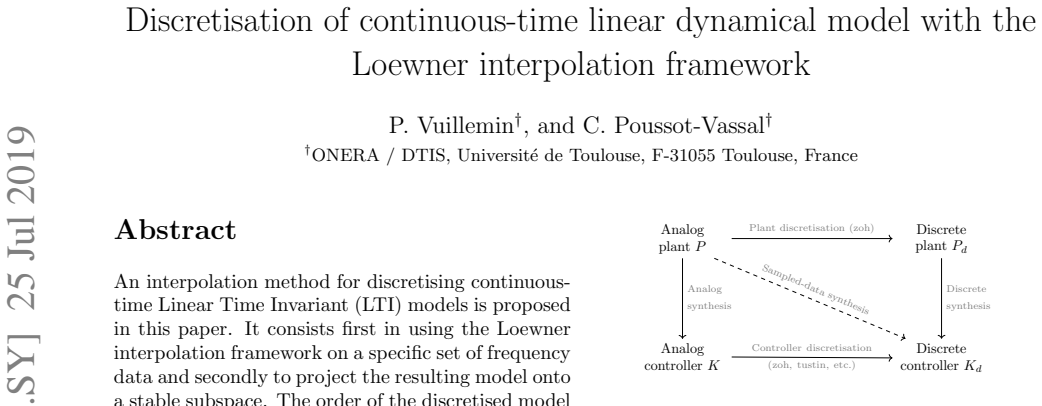
An interpolation method for discretising continuous-time Linear Time Invariant (LTI) models is proposed in this paper. It consists first in using the Loewner interpolation framework on a specific set of frequency data and secondly to project the resulting model onto a stable subspace. The order of the discretised model may be chosen larger than the initial one thus allowing for trading complexity for accuracy if needed. Numerical examples highlight the efficiency of the method at preserving a satisfactory matching both in magnitude and phase in comparison to standard discretisation methods like ZOH or Tustin.
What carries the argument
Loewner interpolation framework applied to frequency data of the continuous-time model, followed by projection onto the stable subspace.
If this is right
- The discrete model can be made to match the continuous frequency response in both magnitude and phase more closely than zero-order hold or Tustin approximations.
- Choosing a higher discrete order than the original continuous order improves accuracy at the expense of added states.
- The same frequency-data pipeline works for any continuous LTI model from which frequency samples can be obtained.
- The projection step guarantees stability of the final discrete model without altering the interpolation property at the data points.
Where Pith is reading between the lines
- The method may allow direct use of measured frequency data rather than an analytic continuous model, opening a path to data-driven discretization.
- Higher-order discrete models obtained this way could serve as starting points for model-order reduction in digital controller design.
- Because the approach separates interpolation from stabilization, it might be combined with other projection techniques for constrained discretization problems.
Load-bearing premise
Frequency data taken from the continuous model can be fed to the Loewner framework so that the resulting model, once projected to its stable part, still reproduces the original dynamics even when the discrete order is larger than the continuous order.
What would settle it
A direct comparison showing that the frequency response of the projected discrete model deviates substantially from the continuous model at the chosen interpolation frequencies or in step-response tests.
Figures


read the original abstract
An interpolation method for discretising continuous-time Linear Time Invariant (LTI) models is proposed in this paper. It consists first in using the Loewner interpolation framework on a specific set of frequency data and secondly to project the resulting model onto a stable subspace. The order of the discretised model may be chosen larger than the initial one thus allowing for trading complexity for accuracy if needed. Numerical examples highlight the efficiency of the method at preserving a satisfactory matching both in magnitude and phase in comparison to standard discretisation methods like ZOH or Tustin.
Editorial analysis
A structured set of objections, weighed in public.
Referee Report
Summary. The paper proposes a discretization method for continuous-time LTI systems that first applies the Loewner interpolation framework to a set of frequency samples drawn from the continuous-time model and then projects the resulting discrete-time model onto its stable subspace. The discrete model order may be selected larger than the continuous order to trade complexity for accuracy. Numerical examples are presented to show that the approach achieves better magnitude and phase matching than standard methods such as zero-order hold or Tustin discretization.
Significance. If the empirical performance is shown to be robust and the effect of the stable projection is clarified, the method would supply a data-driven discretization route that permits controlled increase in order for improved fidelity, offering a practical alternative when conventional techniques introduce unacceptable distortion in magnitude or phase.
major comments (2)
- [description of the discretization procedure and projection step] The manuscript provides no analysis of how the stable-subspace projection affects the exact interpolation conditions guaranteed by the Loewner step at the chosen frequencies. Because the projection is applied after interpolation and the discrete order can exceed the continuous order (increasing the chance of unstable modes), the response at the original sample points may change; the central claim of satisfactory matching therefore rests entirely on the numerical examples rather than on preservation of the interpolation property. This appears in the description of the overall procedure and the projection step.
- [numerical examples section] The numerical examples assert superior magnitude/phase matching but supply neither quantitative error metrics (e.g., maximum pointwise error, H-infinity norm of the difference, or integrated squared error) nor explicit criteria for selecting the frequency data points and the projection method. Without these, the generality of the performance claims cannot be evaluated. This appears in the numerical examples section.
minor comments (2)
- The notation used for the frequency data set and the resulting Loewner matrices could be introduced more explicitly to improve readability.
- A short discussion of computational cost scaling with the number of frequency samples would help place the method in context with existing techniques.
Simulated Author's Rebuttal
We thank the referee for the constructive comments. We address each major comment below and indicate planned revisions to strengthen the manuscript.
read point-by-point responses
-
Referee: The manuscript provides no analysis of how the stable-subspace projection affects the exact interpolation conditions guaranteed by the Loewner step at the chosen frequencies. Because the projection is applied after interpolation and the discrete order can exceed the continuous order (increasing the chance of unstable modes), the response at the original sample points may change; the central claim of satisfactory matching therefore rests entirely on the numerical examples rather than on preservation of the interpolation property. This appears in the description of the overall procedure and the projection step.
Authors: We agree that the stable-subspace projection can alter the exact interpolation property at the sampled frequencies. The Loewner framework guarantees interpolation before projection, but the projection is required to ensure a stable discrete-time model, especially when the order is increased beyond the original continuous-time order. While this introduces a potential deviation at the sample points, the numerical examples demonstrate that the overall magnitude and phase matching remains competitive with or superior to standard methods. In the revision we will add a short discussion of this effect, including a brief illustration of the response change before and after projection, to make the trade-off explicit. revision: yes
-
Referee: The numerical examples assert superior magnitude/phase matching but supply neither quantitative error metrics (e.g., maximum pointwise error, H-infinity norm of the difference, or integrated squared error) nor explicit criteria for selecting the frequency data points and the projection method. Without these, the generality of the performance claims cannot be evaluated. This appears in the numerical examples section.
Authors: We concur that quantitative metrics and explicit selection criteria would improve the evaluation. In the revised numerical examples we will report the maximum pointwise error in magnitude and phase, the H-infinity norm of the difference between the original and discretized models, and the integrated squared error over the frequency grid. We will also document the frequency-point selection procedure (logarithmically spaced samples over the bandwidth of interest) and the precise stable-subspace projection algorithm used. revision: yes
Circularity Check
No circularity: standard Loewner application plus projection, validated empirically
full rationale
The paper applies the established Loewner interpolation framework to frequency samples drawn from the continuous-time model, then performs a stable-subspace projection. Neither step is defined in terms of the other, nor is any output quantity fitted to data and then relabeled as a prediction. No self-citation is invoked as a load-bearing uniqueness theorem, and the numerical examples serve as external validation rather than tautological confirmation. The derivation chain therefore remains independent of its own outputs.
Axiom & Free-Parameter Ledger
Reference graph
Works this paper leans on
- [1]
-
[2]
K.J. ˚Astr¨ om and B. Wittenmark. Computer- controlled systems: theory and design . Courier Corporation, 2013
work page 2013
- [3]
-
[4]
T. Chen and B.A. Francis. Input-output stabil- ity of sampled-data systems. IEEE Transactions on Automatic Control, 36(1):50–58, 1991
work page 1991
-
[5]
T. Chen and B.A. Francis. Optimal sampled- data control systems . Springer Science & Busi- ness Media, 1995
work page 1995
-
[6]
K. Glover. All Optimal Hankel Norm Approx- imation of Linear Multivariable Systems, and TheirL∞ error Bounds. International Journal Control, 39(6):1145–1193, 1984
work page 1984
-
[7]
I.V. Gosea and A.C. Antoulas. Stability pre- serving post-processing methods applied in the loewner framework. In Workshop on Signal and Power Integrity, pages 1–4, 2016
work page 2016
- [8]
-
[9]
M. Kohler. On the closest stable descriptor sys- tem in the respective spaces RH2 andRH∞. Linear Algebra and its Applications , 443:34–49, 2014
work page 2014
- [10]
-
[11]
J. Mari. Modifications of rational transfer ma- trices to achieve positive realness. Signal Pro- cessing, 80(4):615–635, 2000
work page 2000
-
[12]
A J. Mayo and A C. Antoulas. A framework for the solution of the generalized realization problem. Linear Algebra and its Applications , 425(2):634–662, 2007
work page 2007
- [13]
-
[14]
P. Schulze and B. Unger. Data-driven interpola- tion of dynamical systems with delay. Systems & Control Letters, 97:125 – 131, 2016. 11
work page 2016
discussion (0)
Sign in with ORCID, Apple, or X to comment. Anyone can read and Pith papers without signing in.