Wide-angle redshift-space distortions at quasi-linear scales: cross-correlation functions from Zel'dovich approximation

Atsushi Taruya; Michel-Andr\`es Breton; Shohei Saga; Tomohiro Fujita; Yann Rasera

Wide-angle redshift-space distortions at quasi-linear scales: cross-correlation functions from Zel'dovich approximation

T0 review · 0 major / 4 minor · reviewed 2026-08-14 · deepseek-v4-flash

Challenge this review Re-run · record.json Download PDF Read on arXiv ↗ Review JSON

Pith's one-line read This paper uses the Zel'dovich approximation to compute the wide-angle redshift-space cross-correlation function at quasi-linear scales, reproducing linear theory and matching N-body dipole and octupole measurements.

desk verdict A careful, self-contained quasi-linear (Zel'dovich) framework for wide-angle RSD cross-correlations, with the selection-function terms Castorina & White dropped; the uniform-radial-selection scope condition is explicit and limits direct survey application, but the paper is solid and deserves a serious referee. read the letter →

arxiv 1908.03854 v2 pith:XYFBZBFZ submitted 2019-08-11 astro-ph.CO

Atsushi Taruya , Shohei Saga , Michel-Andrès Breton , Yann Rasera , Tomohiro Fujita This is my paper · ORCID

classification astro-ph.CO

keywords wide-angleredshift-spacedistortionsZel'dovichapproximationcross-correlationfunctionoddmultipolesquasi-linearscalesselectionLagrangianperturbationtheorylarge-scalestructure

verification ladder T0 review T1 audit T2 compute T3 formal

The pith

A machine-rendered reading of the paper's core claim, the machinery that carries it, and where it could break.

The reading

Redshift-space distortions break both the isotropy and homogeneity of the observed galaxy distribution, and the wide-angle part, usually neglected in the plane-parallel approximation, will bias next-generation surveys. This paper extends the study of wide-angle RSD from linear theory into the quasi-linear regime by adopting the Zel'dovich approximation and computing the cross-correlation function between two differently biased populations. The formalism reproduces the known linear-theory wide-angle result and produces non-zero odd multipoles whose amplitude is set by the difference in bias. Comparison with full-sky N-body simulations shows that the predicted dipole and octupole match the measured signals, and that the radial selection-function term is essential for getting the dipole right. The framework is explicitly built to be extended to relativistic corrections such as gravitational redshift.

What carries the argument

The load-bearing object is the pair correlation integral: $D_{XY}(s_1,s_2)$ from Eq. (18) is a six-dimensional Gaussian integral over Lagrangian pair positions $(\mathbf q_1,\mathbf q_2)$, with covariance $A_{ab}$ built from the displacement auto-covariance $A_{ij}(q) = \langle \Psi^{(S)}_i \Psi^{(S)}_j\rangle$ and cross-covariance $B_{ij}(q_1,q_2) = \langle \Psi^{(S)}_i(\mathbf q_1)\Psi^{(S)}_j(\mathbf q_2)\rangle$, plus bias-weighted vectors $U_a$ and matrix $W_{ab}$; $R_X(s)$ is the corresponding three-dimensional normalization integral. The Zel'dovich approximation, first-order Lagrangian perturbation theory, expresses the redshift-space displacement as $\Psi^{(S)}_i = (\delta_{ij} + f\,\hat q_i\hat q_j)\Psi_j$ with $\nabla\cdot\Psi = -\delta_L$ and $\mathbf v = aH f\,\Psi$, where $f$ is the linear growth rate. That projection makes the displacement statistics position-dependent, which is exactly what carries the wide-angle geometry into the Gaussian integrals.

What would settle it

Measure the wide-angle dipole and octupole cross-correlations in a survey or simulation whose radial selection function is strongly non-uniform, and compare against the same formalism with $\alpha(r) = 2 + d\ln\varphi/d\ln r$ replacing the constant $2$ in the selection term; the predicted dipole changes sign and amplitude in a specific way, so agreement or disagreement with the measured signal would settle whether the uniform-selection assumption is the load-bearing limitation.

Watch

Extended reading notes

Core claim

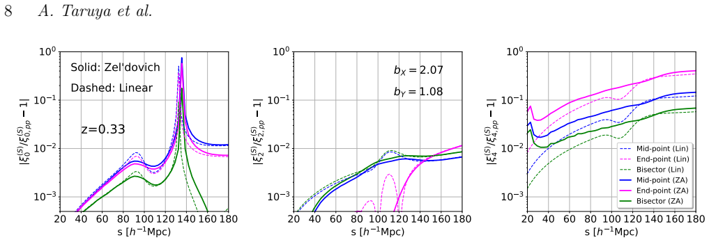
At quasi-linear scales, the wide-angle redshift-space cross-correlation function can be written as the ratio of a six-dimensional Gaussian integral, Eq. (18), to a product of three-dimensional normalization integrals, Eq. (15). These integrals retain the full observer geometry through a position-dependent projection matrix $R_{ij}(\hat q) = \delta_{ij} + f\,\hat q_i \hat q_j$ in the Zel'dovich displacement mapping, so they include all Newtonian wide-angle terms that appear under a uniform radial selection function, including the $(2/s)(\mathbf v\cdot\hat s)$ selection term. Expanding to leading order recovers the standard linear-theory wide-angle RSD formula, and at quasi-linear scales the model matches the dipole and octupole cross-correlations measured from full-sky N-body halo catalogs. The odd multipoles, which vanish in the plane-parallel limit, are proportional to $(b_X-b_Y)$ and are sensitive to the line-of-sight definition, with the end-point definition giving a dipole of opposite sign to the mid-point and bisector definitions.

Load-bearing premise

The derivation assumes the mean number density of each tracer is constant along the line of sight, fixing the radial selection-function term to $(2/s)(\mathbf v\cdot\hat s)$; real surveys have $\alpha(r) = 2 + d\ln\varphi/d\ln r$, and the predicted wide-angle dipole is sensitive to that replacement.

Editorial extensions

If this is right

Wide-angle RSD can now be predicted quasi-linearly for cross-correlations between differently biased tracers with a single set of integral expressions that reduce to linear theory in the appropriate limit.
The wide-angle correction grows with separation and multipole order: the hexadecapole can deviate from the plane-parallel prediction by tens of percent even at small separations, so future surveys need the full calculation rather than the distant-observer approximation.
Odd multipoles in cross-correlations are a real, predictable signal: their amplitude is set by the bias difference and their sign depends on the line-of-sight definition, making them usable as tests of bias models and survey geometry.
The radial selection-function term is essential for the dipole: dropping it flips the sign of the predicted dipole for $b_X>b_Y$, while including it reproduces the N-body result.
Because the formalism is built around displacement statistics rather than linear density alone, it can be extended to include relativistic corrections and applied to isolate gravitational-redshift signals at quasi-linear scales.

Reading between the lines

Editorial extensions of the paper, not claims the author makes directly.

In a real survey the mean tracer density is not constant, so the factor $2$ in the selection term should become $\alpha(r) = 2 + d\ln\varphi/d\ln r$; the paper's own sensitivity analysis shows the dipole is highly dependent on this term, implying realistic surveys may need the $\alpha(r)$ version to avoid a systematic bias.
The same six-dimensional Gaussian machinery could be adapted to a wide-angle cross-power-spectrum estimator or to an auto-correlation with a non-uniform selection function by generalizing $A_{ab}$ and the normalization $R_X$, though the paper does not work out those extensions.
If odd-multipole measurements reach the precision where linear and Zel'dovich predictions separate, comparing dipole and octupole signals across multiple line-of-sight definitions could help disentangle wide-angle Doppler effects from relativistic gravitational redshift, since the two have different bias and selection-function signatures.

Share X Bluesky LinkedIn Reddit HN

Signed reviews

No signed human review yet.

Editorial analysis

A structured set of objections, weighed in public.

Desk editor's note, referee report, and a circularity audit.

Desk Editor's Note

read the letter

The one thing to know: this is a careful, honest extension of Castorina & White's Zel'dovich wide-angle treatment from auto-correlation to cross-correlation. What is actually new is that it keeps all Newtonian wide-angle terms, including the radial selection-function contribution, and it shows—correctly, I think—that the earlier treatment misses the (2/s)(v·s-hat) term. The derivation is thorough: the 3D/6D Gaussian-integral machinery in Eqs. (15) and (18), the linear-theory recovery in Appendix C, and the analytic LOS-dependent multipole formulas in Appendix D are all explicit. The N-body comparison in Fig. 6 uses external bias inputs, so there is no circularity. The paper is also honest that within jackknife errors, linear theory fits the measured dipole and octupole about as well as Zel'dovich does; the quasi-linear advantage is not demonstrated at the scales tested. That is a limitation of the test, not a misrepresentation.

The genuine soft spot is the uniform radial selection function. It is an explicit scope condition: constant mean density in Eq. (9), fixed coefficient 2/s in Eq. (23). The paper's own Sec. 3.3.2 shows the predicted dipole is largely controlled by this term, and that the octupole is insensitive to it. Real surveys have alpha(r) = 2 + d ln phi / d ln r, so direct application to observational data will need extension. The authors say this themselves; it is a stated boundary, not a hidden error. The other mild weakness is that the main motivation—that Zel'dovich matters for quasi-linear scales—is deferred to the companion paper on relativistic corrections. Here, the comparison is not discriminating.

I checked the appendices for internal consistency (the cumulant expansion, the Gaussian identities, the tripolar harmonics coefficient matching). It all hangs together. The complaint that it is incremental relative to Castorina & White is fair but minor: the missing selection-function term matters quantitatively, and the cross-correlation case generates odd multipoles that are absent in auto-correlation.

Who is this for? Theorists and analysts working on wide-angle RSD, odd multipoles, and relativistic corrections in next-generation surveys. It deserves a serious referee: the algebra is dense but checkable, the comparison is fair, and the paper will be the reference for the follow-up. Recommend accept. I would not insist on more N-body discrimination before publication, but I would ask the authors to state explicitly in the abstract or conclusions that the uniform-selection assumption must be relaxed for real surveys.

Referee Report

0 major / 4 minor

Summary. The paper presents a quasi-linear, wide-angle redshift-space distortion model for the cross-correlation function between two biased tracers. It derives the redshift-space density from number conservation under the Zel'dovich approximation, obtains a 3D Gaussian integral for the mean-density normalisation R_X and a 6D Gaussian integral for the pair term D_XY (Eqs. 15 and 18), and shows by Taylor expansion that the linear limit reproduces the standard wide-angle RSD result (Eq. C12) under a uniform radial selection function. It then studies the magnitude of wide-angle corrections as a function of separation, redshift, bias, and line-of-sight definition, and compares dipole and octupole predictions with full-sky N-body halo catalogs. The N-body comparison shows agreement within jackknife errors but does not clearly favour Zel'dovich over linear theory. The paper is explicit that the uniform-selection-function assumption is a scope condition and that extension to non-uniform selection is left to future work.

Significance. If correct, this is the first complete Zel'dovich-level treatment of wide-angle RSD in cross-correlation that includes all Newtonian terms, not just the radial-projection term considered by Castorina & White (2018b). The derivation is self-contained and checkable: the Gaussian integrals in Appendix A, the linear-theory recovery in Appendix C, and the multipole formulas in Appendix D are explicit. The paper also avoids fitting to the target signal: bias parameters are taken from external auto-correlation measurements, and the linear limit is used as a consistency check. The main caveats are the uniform radial selection function and the fact that the N-body validation cannot statistically distinguish the Zel'dovich prediction from linear theory; both are acknowledged in the text. These caveats limit immediate applicability but do not undermine the central derivation.

minor comments (4)

[Abstract; Sec. 2.2] The abstract promises a quasi-linear treatment of wide-angle RSD without stating the uniform radial selection function; given the sensitivity of the dipole to this term shown in Eq. (37), the abstract should mention this scope condition explicitly.
[Fig. 6; Sec. 3.3.1] The line-style assignment is described inconsistently: the text first says 'analytical predictions with Zel'dovich approximation are plotted in magenta solid lines' and then says 'predictions based on linear theory and Zel'dovich approximation are shown in magenta solid and black dashed lines, respectively.' The legend should be made unambiguous.
[Eq. (C8)] The denominator is written R_X(s1)R_X(s2), whereas Eq. (12) has R_X(s1)R_Y(s2); because the two functions are shown equal this is harmless, but the notation should be corrected for consistency.
[App. D2.3, Eqs. (D44)-(D46)] The second displayed expression is labelled bisect ξ_0,2 again, but the right-hand side is the quadrupole contribution; the label should be ξ_2,2 to match the ordering of the even-multipole results.

Circularity Check

0 steps flagged · score 0.0 of 10

No circularity: the quasi-linear wide-angle cross-correlation calculation is a self-contained derivation from the Zel'dovich mapping; the only measured inputs are external bias parameters not fitted to the predicted dipole/octupole.

full rationale

The paper's derivation chain is self-contained. It starts from the standard redshift-space mapping s = x + (1/aH)(v·xhat)xhat (Eq. 1) and the Zel'dovich displacement relation (Eq. 5), then obtains the Gaussian-integral forms for R_X and D_XY (Eqs. 15 and 18) by explicit analytical integration. The inputs are the linear power spectrum, the linear growth rate f, and the bias parameters; no quantity that is later called a prediction is fitted from the target cross-correlation signal. The bias values used in Fig. 6 are taken from the auto-correlation measurements of the same halo catalog in Breton et al. (2019), which is an external calibration and not a fit to the dipole/octupole cross-correlation being compared. The claimed recovery of linear wide-angle RSD (Eq. 23 and Appendix C) is a mathematical limit of the same formalism, not an independent forecast or a renamed input. The uniform-radial-selection-function assumption is explicitly stated (after Eq. 9) and its sensitivity is analyzed in Sec. 3.3.2, so it is a scope condition rather than a hidden circular loop. Self-citations to Castorina & White (2018b) and Breton et al. (2019) are used as prior modeling choices and simulation data, not as a uniqueness theorem or as authority that forces the present result. Therefore no circular step is present.

Assumptions & free parameters 2 free parameters · 5 assumptions · 0 invented entities

The numerical predictions depend on two externally measured bias parameters and on standard cosmological inputs; the formalism itself introduces no new free parameters or invented entities. The dominant assumptions are the Zel'dovich mapping, Gaussian initial conditions, linear bias with no velocity bias, and a uniform selection function.

free parameters (2)

Eulerian linear bias of tracer X, b_X = 2.07
Measured from the halo auto-correlation in Breton et al. (2019), Table 2; used as input to the cross-correlation predictions, not fitted to the target signal.
Eulerian linear bias of tracer Y, b_Y = 1.08 (also 1.69 in the lower panel)
Same external measurement; the odd multipole amplitude is proportional to b_X minus b_Y.

assumptions (5)

domain assumption Initial linear density field delta_L is Gaussian and statistically homogeneous and isotropic in Lagrangian space.
Used throughout Sec. 2.2 and Appendix A to evaluate Gaussian integrals and cumulant expansions; primordial non-Gaussianity is neglected.
domain assumption Zel'dovich approximation: x = q + Psi with div Psi = -delta_L and v = a H f Psi.
Defines the quasi-linear model; no second-order displacement, vorticity, or additional stress terms are included.
domain assumption The line-of-sight direction in the redshift-space displacement is evaluated at the Lagrangian position: x-hat approximately equals q-hat in Eq. (8).
Valid to first order in Lagrangian perturbation theory; it makes the mapping and the position-dependent matrix R tractable.
domain assumption Linear Lagrangian bias relation and no velocity bias: n_X proportional to 1 + b^L_X delta_L(q), and objects follow the matter velocity flow.
Eq. (9) and Sec. 2.1; nonlinear or stochastic bias and velocity bias are excluded.
domain assumption Uniform radial selection function with constant mean number density.
Sec. 2.2 and Sec. 2.3; replaces the general alpha(r) with 2 in Eq. (23), and is key for the dipole prediction.

how reviews work

0 comments

Cite this review

Pith. "Pith review of Wide-angle redshift-space distortions at quasi-linear scales: cross-correlation functions from Zel'dovich approximation." pith.science (2026). https://pith.science/paper/XYFBZBFZ

@misc{pith2026190803854,
  author       = {Pith},
  title        = {Pith review of: Wide-angle redshift-space distortions at quasi-linear scales: cross-correlation functions from Zel'dovich approximation},
  year         = {2026},
  howpublished = {\url{https://pith.science/paper/XYFBZBFZ}},
  note         = {Machine review of arXiv:1908.03854}
}

read the original abstract

Redshift-space distortions (RSD) in galaxy redshift surveys generally break both the isotropy and homogeneity of galaxy distribution. While the former aspect is particularly highlighted as a probe of growth of structure induced by gravity, the latter aspect, often quoted as wide-angle RSD but ignored in most of the cases, will become important and critical to account for as increasing the statistical precision in next-generation surveys. However, the impact of wide-angle RSD has been mostly studied using linear perturbation theory. In this paper, employing the Zel'dovich approximation, i.e., first-order Lagrangian perturbation theory for gravitational evolution of matter fluctuations, we present a quasi-linear treatment of wide-angle RSD, and compute the cross-correlation function. The present formalism consistently reproduces linear theory results, and can be easily extended to incorporate relativistic corrections (e.g., gravitational redshift).

Figures

Figures reproduced from arXiv: 1908.03854 by the authors.

**Figure 1.** Geometric configuration of redshift-space crosscorrelation function. Along the line-of-sight direction d, a pair of objects X and Y is found at the positions s1 and s2, where the density fields, denoted by δ (S) X and δ (S) Y , is measured. The separation between these two objects is defined by s ≡ s2 − s1. Misalignment between s and d is characterized by the angle ϕ or the directional cosine given by µ ≡ cos ϕ. No… view at source ↗

**Figure 2.** Fractional difference of the monopole (left), quadrupole (middle), and hexadecapole (right) moments of correlation function between predictions with and without wide-angle effects, |ξ (S) ` /ξ(S) `,pp − 1|, where ξ (S) `,pp represents the multipole correlation function in the plane-parallel limit. The results at z = 0.1, 0.33, and 0.57 are shown in different colors. Solid and dashed lines are respectively the predic… view at source ↗

**Figure 3.** Dipole (left) and Octupole (right) moments of cross-correlation function at z = 0.1 (black), 0.33 (green), and 0.57 (blue). The plotted results are the multipole correlation function multiplied by s 2 . Solid and dashed lines are the predictions based on Zel’dovich approximation and linear theory, respectively. Same as in [PITH_FULL_IMAGE:figures/full_fig_p007_3.png] view at source ↗

Figures from the paper (3 more)

**Figure 4.** Figure 4: Dependence of monopole (left), quadrupole (middle), and hexadecapole (right) cross-correlation functions on the LOS definition at z = 0.33. Same as in [PITH_FULL_IMAGE:figures/full_fig_p008_4.png]

**Figure 5.** Figure 5: Dependence of LOS definition on dipole (left) and octupole (right) moments of cross-correlation functions at z = 0.33. The plotted results are the multipole correlation function multiplied by s 2 , assuming the Eulerian linear bias of bX = 2.07 and bY = 1.08. Meanings …

**Figure 6.** Figure 6: Comparison of the dipole (left) and octupole (right) moments of cross-correlation function between analytical predictions and measured results in N-body simulations, adopting the mid-point LOS given at Eq. (29). Upper and lower panels shows the results for the halos wi…

Discussion (0). Continue with ORCID to comment.

Forward citations

Cited by 1 Pith paper

Reviewed papers in the Pith corpus that reference this work. Sorted by Pith novelty score. Full citation record

Gravitational redshift from large-scale structure: nonlinearities, antisymmetries, and the dipole
astro-ph.CO 2025-06 conditional novelty 6.0 of 10

A wide-angle streaming model including gravitational redshift, lightcone and kinematic effects explains the dipole turnover at ~20 h^-1 Mpc as an advection-like shift driven by the density-weighted pairwise potential ...

Reference graph

Works this paper leans on

64 extracted references · 14 canonical work pages · cited by 1 Pith paper

[1]

Alam S., Zhu H., Croft R. A. C., Ho S., Giusarma E., Schneider D. P., 2017a, @doi [ ] 10.1093/mnras/stx1421 , http://adsabs.harvard.edu/abs/2017MNRAS.470.2822A 470, 2822

doi:10.1093/mnras/stx1421
[2]

Alam S., et al., 2017b, @doi [ ] 10.1093/mnras/stx721 , https://ui.adsabs.harvard.edu/abs/2017MNRAS.470.2617A 470, 2617

doi:10.1093/mnras/stx721
[3]

Bertacca D., Maartens R., Raccanelli A., Clarkson C., 2012, @doi [ ] 10.1088/1475-7516/2012/10/025 , https://ui.adsabs.harvard.edu/abs/2012JCAP...10..025B 2012, 025

doi:10.1088/1475-7516/2012/10/025 2012
[4]

Beutler F., et al., 2014, @doi [ ] 10.1093/mnras/stu1051 , https://ui.adsabs.harvard.edu/abs/2014MNRAS.443.1065B 443, 1065

doi:10.1093/mnras/stu1051 2014
[5]

Beutler F., Castorina E., Zhang P., 2019, @doi [Journal of Cosmology and Astro-Particle Physics] 10.1088/1475-7516/2019/03/040 , https://ui.adsabs.harvard.edu/abs/2019JCAP...03..040B 2019, 040

doi:10.1088/1475-7516/2019/03/040 2019
[6]

J., 2015, @doi [Monthly Notices of the Royal Astronomical Society: Letters] 10.1093/mnrasl/slv090 , 453, L11

Bianchi D., Gil-Mar \' i n H., Ruggeri R., Percival W. J., 2015, @doi [Monthly Notices of the Royal Astronomical Society: Letters] 10.1093/mnrasl/slv090 , 453, L11

doi:10.1093/mnrasl/slv090 2015
[7]

Bond J., Couchman H., 1988, in The Post-Recombination Universe , Proceedings of the NATO Advanced Study Institute, Kluwer Academic Publishers, p.263

work page 1988
[8]

Bonvin C., Durrer R., 2011, @doi [ ] 10.1103/PhysRevD.84.063505 , http://adsabs.harvard.edu/abs/2011PhRvD..84f3505B 84, 063505

doi:10.1103/physrevd.84.063505 2011

Show all 64 references

[9]

Bonvin C., Hui L., Gazta \ n aga E., 2014, @doi [ ] 10.1103/PhysRevD.89.083535 , http://adsabs.harvard.edu/abs/2014PhRvD..89h3535B 89, 083535

2014 doi
[10]

Breton M.-A., Rasera Y., Taruya A., Lacombe O., Saga S., 2019, @doi [ ] 10.1093/mnras/sty3206 , http://adsabs.harvard.edu/abs/2019MNRAS.483.2671B 483, 2671

2019 doi
[11]

Carlson J., Reid B., White M., 2013, @doi [ ] 10.1093/mnras/sts457 , https://ui.adsabs.harvard.edu/abs/2013MNRAS.429.1674C 429, 1674

2013 doi
[12]

Castorina E., White M., 2018a, @doi [ ] 10.1093/mnras/sty410 , http://adsabs.harvard.edu/abs/2018MNRAS.476.4403C 476, 4403

doi
[13]

Castorina E., White M., 2018b, @doi [ ] 10.1093/mnras/sty1437 , http://adsabs.harvard.edu/abs/2018MNRAS.479..741C 479, 741

doi
[14]

Challinor A., Lewis A., 2011, @doi [ ] 10.1103/PhysRevD.84.043516 , http://adsabs.harvard.edu/abs/2011PhRvD..84d3516C 84, 043516

2011 doi
[15]

Crocce M., Scoccimarro R., 2008, @doi [ ] 10.1103/PhysRevD.77.023533 , 77, 023533

2008 doi
[16]

Di Dio E., Seljak U., 2019, @doi [ ] 10.1088/1475-7516/2019/04/050 , https://ui.adsabs.harvard.edu/abs/2019JCAP...04..050D 2019, 050

2019 doi
[17]

B., Nusser A., 1996, @doi [ ] 10.1093/mnras/279.1.L1 , https://ui.adsabs.harvard.edu/abs/1996MNRAS.279L...1F 279, L1

Fisher K. B., Nusser A., 1996, @doi [ ] 10.1093/mnras/279.1.L1 , https://ui.adsabs.harvard.edu/abs/1996MNRAS.279L...1F 279, L1

1996 doi
[18]

B., Scharf C

Fisher K. B., Scharf C. A., Lahav O., 1994, @doi [ ] 10.1093/mnras/266.1.219 , https://ui.adsabs.harvard.edu/\#abs/1994MNRAS.266..219F 266, 219

1994 doi
[19]

Gaztanaga E., Bonvin C., Hui L., 2017, @doi [ ] 10.1088/1475-7516/2017/01/032 , http://adsabs.harvard.edu/abs/2017JCAP...01..032G 1, 032

2017 doi
[20]

Hahn T., 2005, @doi [Comput. Phys. Commun.] 10.1016/j.cpc.2005.01.010 , 168, 78

2005 doi
[21]

Hamilton A. J. S., 1992, @doi [Astrophys. J.] 10.1086/186264 , http://ads.nao.ac.jp/abs/1992ApJ...385L...5H 385, L5

1992 doi
[22]

Hamilton A. J. S., Culhane M., 1996, @doi [ ] 10.1093/mnras/278.1.73 , http://adsabs.harvard.edu/abs/1996MNRAS.278...73H 278, 73

1996 doi
[23]

F., Taylor A

Heavens A. F., Taylor A. N., 1995, @doi [ ] 10.1093/mnras/275.2.483 , http://adsabs.harvard.edu/abs/1995MNRAS.275..483H 275, 483

1995 doi
[24]

Kaiser N., 1987, @doi [ ] 10.1093/mnras/227.1.1 , https://ui.adsabs.harvard.edu/abs/1987MNRAS.227....1K 227, 1

1987 doi
[25]

Komatsu E., et al., 2011, @doi [ ] 10.1088/0067-0049/192/2/18 , https://ui.adsabs.harvard.edu/abs/2011ApJS..192...18K 192, 18

2011 doi
[26]

J.] 10.1086/309179 , 538, 473

Lewis A., Challinor A., Lasenby A., 2000, @doi [Astrophys. J.] 10.1086/309179 , 538, 473

2000 doi
[27]

V., 2008, @doi [Astropart

Linder E. V., 2008, @doi [Astropart. Phys.] 10.1016/j.astropartphys.2008.03.002 , 29, 336

2008 doi
[28]

Matsubara T., 2000, @doi [ ] 10.1086/308827 , http://adsabs.harvard.edu/abs/2000ApJ...535....1M 535, 1

2000 doi
[29]

Matsubara T., 2008a, @doi [ ] 10.1103/PhysRevD.77.063530 , 77, 063530

doi
[30]

Matsubara T., 2008b, @doi [ ] 10.1103/PhysRevD.78.083519 , 78, 083519

doi
[31]

Matsubara T., 2014, @doi [ ] 10.1103/PhysRevD.90.043537 , https://ui.adsabs.harvard.edu/abs/2014PhRvD..90d3537M 90, 043537

2014 doi
[32]

S., Landy S

Matsubara T., Szalay A. S., Landy S. D., 2000, @doi [ ] 10.1086/312701 , https://ui.adsabs.harvard.edu/abs/2000ApJ...535L...1M 535, L1

2000 doi
[33]

McDonald P., 2009, @doi [Journal of Cosmology and Astro-Particle Physics] 10.1088/1475-7516/2009/11/026 , https://ui.adsabs.harvard.edu/abs/2009JCAP...11..026M 2009, 026

2009 doi
[34]

A., 1969, Soviet Journal of Experimental and Theoretical Physics, http://adsabs.harvard.edu/abs/1969JETP...30..512N 30, 512

Novikov E. A., 1969, Soviet Journal of Experimental and Theoretical Physics, http://adsabs.harvard.edu/abs/1969JETP...30..512N 30, 512

1969
[35]

J., Kayo I., Hikage C., Szalay A

Okumura T., Matsubara T., Eisenstein D. J., Kayo I., Hikage C., Szalay A. S., Schneider D. P., 2008, @doi [ ] 10.1086/528951 , https://ui.adsabs.harvard.edu/\#abs/2008ApJ...676..889O 676, 889

2008 doi
[36]

P \'a pai P., Szapudi I., 2008, @doi [ ] 10.1111/j.1365-2966.2008.13572.x , http://adsabs.harvard.edu/abs/2008MNRAS.389..292P 389, 292

2008
[37]

J., White M., 2009, , 393, 297

Percival W. J., White M., 2009, , 393, 297

2009
[38]

C., et al., 2004, @doi [ ] 10.1086/383533 , https://ui.adsabs.harvard.edu/abs/2004ApJ...607..655P 607, 655

Pope A. C., et al., 2004, @doi [ ] 10.1086/383533 , https://ui.adsabs.harvard.edu/abs/2004ApJ...607..655P 607, 655

2004 doi
[39]

J., 2010, @doi [ ] 10.1111/j.1365-2966.2010.17388.x , https://ui.adsabs.harvard.edu/abs/2010MNRAS.409.1525R 409, 1525

Raccanelli A., Samushia L., Percival W. J., 2010, @doi [ ] 10.1111/j.1365-2966.2010.17388.x , https://ui.adsabs.harvard.edu/abs/2010MNRAS.409.1525R 409, 1525

2010
[40]

C., Szalay A

Raccanelli A., Bertacca D., Jeong D., Neyrinck M. C., Szalay A. S., 2018, @doi [Physics of the Dark Universe] 10.1016/j.dark.2017.12.003 , https://ui.adsabs.harvard.edu/abs/2018PDU....19..109R 19, 109

2018 doi
[41]

Reimberg P., Bernardeau F., Pitrou C., 2016, @doi [ ] 10.1088/1475-7516/2016/01/048 , http://adsabs.harvard.edu/abs/2016JCAP...01..048R 1, 048

2016 doi
[42]

Schneider P., Bartelmann M., 1995, @doi [ ] 10.1093/mnras/273.2.475 , https://ui.adsabs.harvard.edu/abs/1995MNRAS.273..475S 273, 475

1995 doi
[43]

Scoccimarro R., 2004, @doi [ ] 10.1103/PhysRevD.70.083007 , 70, 083007

2004 doi
[44]

Scoccimarro R., 2015, @doi [Physical Review D] 10.1103/PhysRevD.92.083532 , 92, 1

2015 doi
[45]

F., Zeldovich Y

Shandarin S. F., Zeldovich Y. B., 1989, @doi [Reviews of Modern Physics] 10.1103/RevModPhys.61.185 , http://adsabs.harvard.edu/abs/1989RvMP...61..185S 61, 185

1989 doi
[46]

R., Lewis A., 2008, @doi [ ] 10.1103/PhysRevD.78.103512 , 78, 103512

Shaw J. R., Lewis A., 2008, @doi [ ] 10.1103/PhysRevD.78.103512 , 78, 103512

2008 doi
[47]

J., 2009, @doi [ ] 10.1088/1475-7516/2009/10/004 , 0910, 004

Song Y.-S., Percival W. J., 2009, @doi [ ] 10.1088/1475-7516/2009/10/004 , 0910, 004

2009 doi
[48]

S., Matsubara T., Landy S

Szalay A. S., Matsubara T., Landy S. D., 1998, @doi [ ] 10.1086/311293 , http://adsabs.harvard.edu/abs/1998ApJ...498L...1S 498, L1

1998 doi
[49]

Szapudi I., 2004, @doi [ ] 10.1086/423168 , http://adsabs.harvard.edu/abs/2004ApJ...614...51S 614, 51

2004 doi
[50]

Tadros H., et al., 1999, @doi [ ] 10.1046/j.1365-8711.1999.02409.x , https://ui.adsabs.harvard.edu/abs/1999MNRAS.305..527T 305, 527

1999
[51]

Tansella V., Bonvin C., Durrer R., Ghosh B., Sellentin E., 2018, @doi [ ] 10.1088/1475-7516/2018/03/019 , https://ui.adsabs.harvard.edu/abs/2018JCAP...03..019T 2018, 019

2018 doi
[52]

Taruya A., Nishimichi T., Saito S., Hiramatsu T., 2009, @doi [ ] 10.1103/PhysRevD.80.123503 , 80, 123503

2009 doi
[53]

Taruya A., Nishimichi T., Saito S., 2010, @doi [ ] 10.1103/PhysRevD.82.063522 , 82, 063522

2010 doi
[54]

N., Hamilton A

Taylor A. N., Hamilton A. J. S., 1996, @doi [ ] 10.1093/mnras/282.3.767 , https://ui.adsabs.harvard.edu/abs/1996MNRAS.282..767T 282, 767

1996 doi
[55]

Vlah Z., Seljak U., McDonald P., Okumura T., Baldauf T., 2012, @doi [ ] 10.1088/1475-7516/2012/11/009 , 1211, 009

2012 doi
[56]

Wang L., Reid B., White M., 2014, @doi [ ] 10.1093/mnras/stt1916 , https://ui.adsabs.harvard.edu/abs/2014MNRAS.437..588W 437, 588

2014 doi
[57]

H., Mortonson M

Weinberg D. H., Mortonson M. J., Eisenstein D. J., Hirata C., Riess A. G., Rozo E., 2013, @doi [Phys. Rept.] 10.1016/j.physrep.2013.05.001 , http://adsabs.harvard.edu/abs/2013PhR...530...87W 530, 87

2013 doi
[58]

White M., 2014, @doi [ ] 10.1093/mnras/stu209 , https://ui.adsabs.harvard.edu/abs/2014MNRAS.439.3630W 439, 3630

2014 doi
[59]

Yoo J., 2010, @doi [ ] 10.1103/PhysRevD.82.083508 , https://ui.adsabs.harvard.edu/abs/2010PhRvD..82h3508Y 82, 083508

2010 doi
[60]

Yoo J., Seljak U., 2015, @doi [ ] 10.1093/mnras/stu2491 , http://adsabs.harvard.edu/abs/2015MNRAS.447.1789Y 447, 1789

2015 doi
[61]

L., Zaldarriaga M., 2009, @doi [ ] 10.1103/PhysRevD.80.083514 , https://ui.adsabs.harvard.edu/abs/2009PhRvD..80h3514Y 80, 083514

Yoo J., Fitzpatrick A. L., Zaldarriaga M., 2009, @doi [ ] 10.1103/PhysRevD.80.083514 , https://ui.adsabs.harvard.edu/abs/2009PhRvD..80h3514Y 80, 083514

2009 doi
[62]

Yoo J., Hamaus N., Seljak U., Zaldarriaga M., 2012, @doi [ ] 10.1103/PhysRevD.86.063514 , http://adsabs.harvard.edu/abs/2012PhRvD..86f3514Y 86, 063514

2012 doi
[63]

Zaroubi S., Hoffman Y., 1996, @doi [ ] 10.1086/177124 , http://adsabs.harvard.edu/abs/1996ApJ...462...25Z 462, 25

1996 doi
[64]

B., 1970, , http://adsabs.harvard.edu/abs/1970A

Zel'dovich Y. B., 1970, , http://adsabs.harvard.edu/abs/1970A

1970

Pith tools

Reviewed August 14, 2026 · model on record in the stance chip above.

[1] [1]

Alam S., Zhu H., Croft R. A. C., Ho S., Giusarma E., Schneider D. P., 2017a, @doi [ ] 10.1093/mnras/stx1421 , http://adsabs.harvard.edu/abs/2017MNRAS.470.2822A 470, 2822

doi:10.1093/mnras/stx1421

[2] [2]

Alam S., et al., 2017b, @doi [ ] 10.1093/mnras/stx721 , https://ui.adsabs.harvard.edu/abs/2017MNRAS.470.2617A 470, 2617

doi:10.1093/mnras/stx721

[3] [3]

Bertacca D., Maartens R., Raccanelli A., Clarkson C., 2012, @doi [ ] 10.1088/1475-7516/2012/10/025 , https://ui.adsabs.harvard.edu/abs/2012JCAP...10..025B 2012, 025

doi:10.1088/1475-7516/2012/10/025 2012

[4] [4]

Beutler F., et al., 2014, @doi [ ] 10.1093/mnras/stu1051 , https://ui.adsabs.harvard.edu/abs/2014MNRAS.443.1065B 443, 1065

doi:10.1093/mnras/stu1051 2014

[5] [5]

Beutler F., Castorina E., Zhang P., 2019, @doi [Journal of Cosmology and Astro-Particle Physics] 10.1088/1475-7516/2019/03/040 , https://ui.adsabs.harvard.edu/abs/2019JCAP...03..040B 2019, 040

doi:10.1088/1475-7516/2019/03/040 2019

[6] [6]

J., 2015, @doi [Monthly Notices of the Royal Astronomical Society: Letters] 10.1093/mnrasl/slv090 , 453, L11

Bianchi D., Gil-Mar \' i n H., Ruggeri R., Percival W. J., 2015, @doi [Monthly Notices of the Royal Astronomical Society: Letters] 10.1093/mnrasl/slv090 , 453, L11

doi:10.1093/mnrasl/slv090 2015

[7] [7]

Bond J., Couchman H., 1988, in The Post-Recombination Universe , Proceedings of the NATO Advanced Study Institute, Kluwer Academic Publishers, p.263

work page 1988

[8] [8]

Bonvin C., Durrer R., 2011, @doi [ ] 10.1103/PhysRevD.84.063505 , http://adsabs.harvard.edu/abs/2011PhRvD..84f3505B 84, 063505

doi:10.1103/physrevd.84.063505 2011