Boundary Defense against Cyber Threat for Power System Operation

Javad Lavaei; Ming Jin; Ross Baldick; Somayeh Sojoudi

REVIEW 3 major objections 5 minor 49 references

Boundary Defense against Cyber Threat for Power System Operation

T0 review · 3 major / 5 minor · reviewed 2026-08-14 · deepseek-v4-flash

Challenge this review Re-run · record.json Download PDF Read on arXiv ↗ Review JSON

Pith's one-line read The paper proves that a per-line vulnerability index below one makes a local power-grid cyber attack provably containable.

desk verdict The boundary defense framework is genuinely new and the containment result mostly holds, but the no-false-positives claim in Theorem 1 is not proven by the supplied arguments. read the letter →

arxiv 1908.10315 v1 pith:XZRHUATY submitted 2019-08-04 eess.SP stat.AP

Ming Jin , Javad Lavaei , Somayeh Sojoudi , Ross Baldick This is my paper · ORCID

classification eess.SPstat.AP

keywords powersystemstateestimationcyberattackbaddatadetectionboundarydefensevulnerabilityindexsecond-orderconeprogrammingmutualincoherencegridmap

verification ladder T0 review T1 audit T2 compute T3 formal

The pith

A machine-rendered reading of the paper's core claim, the machinery that carries it, and where it could break.

The reading

Power-system state estimation is usually a nonconvex, nonlinear problem, and standard solvers can fail badly when a few measurements are corrupted. This paper argues that by rewriting all common measurements as linear functions of a new set of variables—voltage magnitudes squared and the real and imaginary parts of phasor products—state estimation becomes a convex problem that can simultaneously estimate the state and detect bad data. Its central result is a containment guarantee for localized attacks: if the vulnerability index of every line on the boundary of an attacked region is below one in the outward direction, then the two-step pipeline produces no false positives in bad-data detection and exactly recovers the state everywhere outside the attacked region. The paper further shows that adding second-order cone constraints never weakens this guarantee, and it maps which lines and substations of a synthetic U.S. grid are vulnerable or critical.

What carries the argument

The carrying mechanism is a change of measurement basis: each bus contributes a voltage-magnitude-squared variable $x^{\mathrm{mg}}_k = |v_k|^2$ and each line contributes $x^{\mathrm{re}}_\ell = \mathrm{Re}(v_i v_j^*)$ and $x^{\mathrm{im}}_\ell = \mathrm{Im}(v_i v_j^*)$, under which every standard power-flow, injection, and voltage-magnitude measurement becomes a linear equation. On top of this basis, the paper defines the line vulnerability index $\alpha_{i\to j} = \max_{\xi\in\{\pm1\}^{n_\times}} \min_{h: \, A^\top_{M_{\checkmark},X_{\mathrm{bd}}}h + A^\top_{M_{\times},X_{\mathrm{bd}}}\xi = 0} \|h\|_\infty$, a minimax quantity that measures whether boundary measurements can dominate arbitrary unit-bounded error patterns on the attacked side of a line. The proof machinery is an induction (Lemma 11, and Lemma 17 for the SOCP case) showing the per-line condition implies the existence of a bounded dual certificate over the whole boundary, which then yields support recovery and exact state recovery outside the attacked region.

What would settle it

On a small standard test grid, choose a zonal attack for which every outward line vulnerability index is computed to be below one, then run the paper's two-step pipeline both as specified and with a single boundary voltage-magnitude measurement additionally corrupted; if the latter run produces a false positive in the safe region or a biased safe-region state estimate, it demonstrates the boundary-trust premise is load-bearing.

Watch

Extended reading notes

Core claim

The paper's main theorem (Theorem 1; Theorems 12 and 19 in the supplement) states the following. Given a partition of the network into attacked, boundary, and safe regions, with bad data confined to the attacked region, suppose the line vulnerability index $\alpha_{i\to j}$ (LP/QP version) or $\alpha_{i\to j}^{\mathrm{SOCP}}$ is less than 1 for every boundary line in the outward direction, and suppose the relevant full-column-rank conditions hold. Then the solution of the proposed $\ell^1$ or $\ell^2/\ell^1$ convex program (with or without SOC constraints) has no false positives in Step 1, and after removing the attacked subgraph, direct recovery in Step 2 reconstructs the true complex voltage state for all buses in the safe and boundary regions. The vulnerability index itself is the optimal value of a minimax program that asks whether boundary measurements can fully counteract the worst-case adversarial error pattern on the attacked side of a line. The theorem is proven by a 'local implies global' induction that builds a dual certificate for the global problem from per-line certificates, together with a primal-dual witness argument for support recovery.

Load-bearing premise

The guarantee collapses if an adversary corrupts even one boundary measurement, because the proof requires all measurements on the boundary ($M_{\mathrm{bi}}$ and $M_{\mathrm{bo}}$) to be attack-free and requires the sensing matrix to have the block-separable structure of Eq. (26), where no measurement depends jointly on attacked and safe variables.

Editorial extensions

If this is right

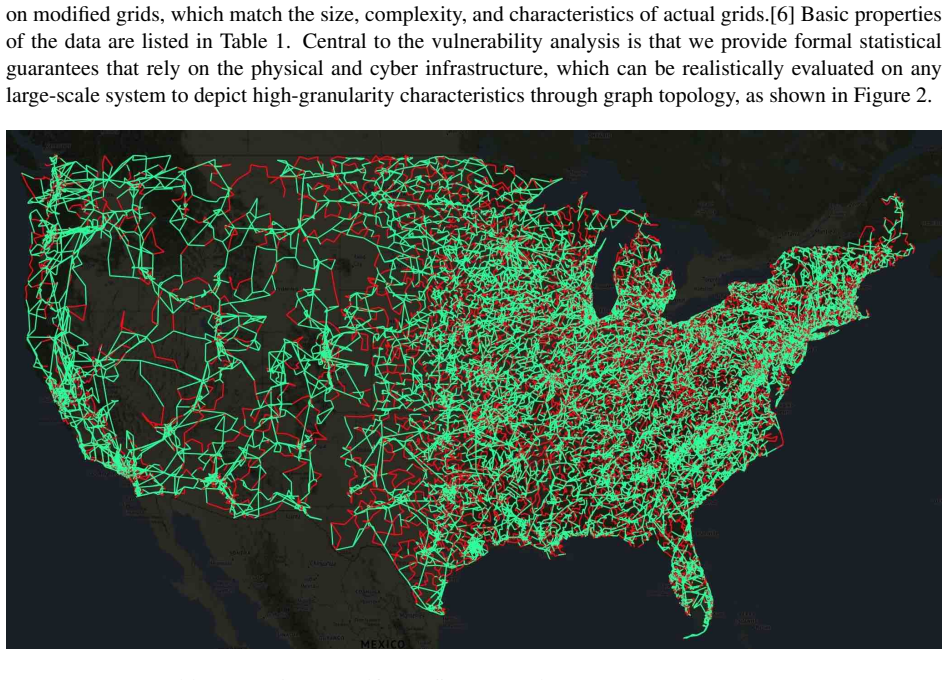
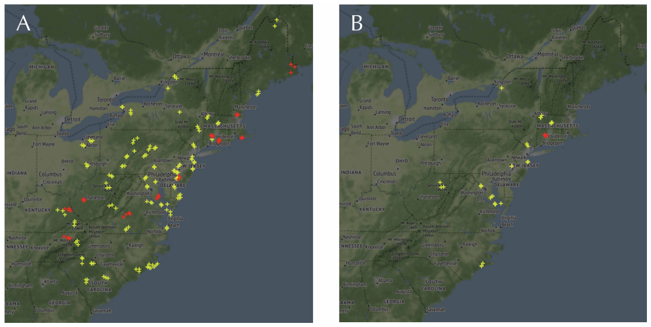
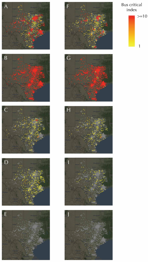
Operators can precompute vulnerability maps offline for a given measurement profile, so before any attack they know which boundaries will contain a zonal corruption and which lines would let an error escape.
The SOCP formulation is never less robust than the LP/QP formulation ($\alpha^{\mathrm{SOCP}}_{i\to j}(x) \le \alpha_{i\to j}$), so adding conic constraints can only expand the set of networks for which the containment guarantee holds.
Measurement hardware choices change the guarantee: adding voltage-magnitude or branch-flow measurements tends to shrink the vulnerable-line set, while adding nodal power-injection measurements tends to enlarge it (Figure 9 and Table 1).
A line or substation surrounded by robust lines is guaranteed to contain topological errors locally, whereas a line with at least one vulnerable outward direction is a critical line through which an error can escape.

Reading between the lines

Editorial extensions of the paper, not claims the author makes directly.

A natural extension the paper does not run: recompute the vulnerability indices online as the active measurement set changes (for example after sensor outages), turning the static map into a dynamic screening tool.
Because the local-to-global induction only needs the block-separable measurement structure of Eq. (26), the same boundary defense guarantee should transfer to other networked sensing problems—water, gas, or transportation—that admit a linear measurement model.
The theorem implies the scarce security resource is boundary measurement integrity; an operator could concentrate hardening on the thin boundary ring rather than on all sensors, a resource-allocation consequence implicit in the paper.

Share X Bluesky LinkedIn Reddit HN

Signed reviews

No signed human review yet.

Editorial analysis

A structured set of objections, weighed in public.

Desk editor's note, referee report, and a circularity audit.

Desk Editor's Note

read the letter

Dear [colleague],

Quick take: this is a real contribution, but the main-text Theorem 1 oversells what the supplementary proofs actually establish. The containment half—recovering the state outside the attacked region when boundary indices are below 1—is largely supported. The no-false-positives half is not, at least not from the supplied arguments.

What's new: the paper reformulates AC power flow measurements in a linear basis and defines per-line vulnerability indices via a minimax condition. The local-to-global induction connecting alpha<1 on all boundary lines to global recovery is a clever idea, and the SOCP version provably dominates the LP/QP version. The vulnerability maps on synthetic US grids are a nice practical output. I'm not aware of prior work with this kind of graph-structured containment certificate for state estimation.

Soft spots, in proportion:

1. The no-false-positive claim. Theorem 1(i) says no false positives in Step 1. The proven Theorems 12 and 19 only recover x_sf and x_bd; they don't control b_hat on Mbi. Since the attacked region's state is unidentifiable, nonzero b_hat on the inner boundary can arise from A_Mbi,Xat (x_at - x_hat_at). In Theorem 13, the primal-dual witness shows strict dual feasibility only on Msf∪Mbo; h_Mbi is just any subgradient, so no-false-inclusion on the inner boundary is not established. This is a genuine gap in the central claim, not a nit.

2. Lemma 11's induction. After setting up cases (shared attack node vs. not, shared outer boundary nodes vs. not), the proof says all combinations reduce to 'two typical scenarios' without full enumeration. There may well be a complete proof hiding there, but as written it's a sketch. Similarly for Lemma 17.

3. The clean-boundary assumption. The entire framework assumes boundary measurements are unattacked and the block-separable structure in Eq. (26). An adversary who corrupts one boundary sensor breaks it. The paper acknowledges this, but worth saying aloud: the guarantee is for algebraic boundary defense, not for an adversary with full access.

What's solid: the GRC condition and vulnerability index are sufficient conditions derived from the sensing matrix, not fitted. The SOCP dominance (Prop 18) is a clean formal result. The empirical comparison to NLS/BDD is reasonable, though no code or error bars. The reliance on the authors' prior work [13] for the AC vulnerability model is fine, since the boundary defense theorems are self-contained.

Who's this for: power system state estimation researchers, and people working on robustness of graph-structured inverse problems. The paper deserves a serious referee. I'd send it to review, with a clear request to fix the mismatch between Theorem 1 and the proven statements—either prove no-false-positives on Mbi, or weaken the main-text claim.

Referee Report

3 major / 5 minor

Summary. The manuscript proposes a robust state estimation framework for AC power systems based on a linear basis of voltage-magnitude squares and phasor products, followed by a two-step pipeline: a convex sparse-bad-data estimator (LP/QP or SOCP) and a phasor-recovery step. It introduces a per-line vulnerability index and claims in Theorem 1 that if all boundary vulnerability indices are below one, then a local (zonal) attack is contained: Step 1 produces no false positives and Step 2 recovers the state outside the attacked region. The paper also provides vulnerability maps for a synthetic U.S. grid, studies the effect of measurement profiles and network topology, and extends the analysis to tree decompositions.

Significance. The paper treats an important and timely problem and contains several valuable ideas: a linear embedding of AC state estimation, a localized per-line vulnerability metric that is provably no more conservative than the global mutual incoherence condition, a proof that SOCP constraints improve the vulnerability index, a scalable formulation of the index via complementarity, and large-scale empirical vulnerability maps. The state-containment half of the main theorem, if fully proved, would be a useful formal guarantee for local attack isolation. However, the advertised 'no false positives' guarantee is not supported by the formal results as written, and the local-to-global induction contains an unresolved gap. These issues affect the central claim and require correction before publication.

major comments (3)

[Theorem 1; Theorems 12/13; Eq. (26)] The no-false-positive claim in Theorem 1(i) is not established. In the noiseless case, Theorem 12 only concludes x̂sf=x♮sf and x̂bd=x♮bd; it does not constrain b̂Mbi. Since b♮Mbi=0 by the clean-boundary assumption in Definitions 3 and 4, any nonzero b̂Mbi is a false positive. From the block structure in Eq. (26), once x̂bd=x♮bd, the Mbi rows force b̂Mbi=A_{Mbi,Xat}(x♮at−x̂at), which need not vanish because x̂at is not identifiable under the stated assumptions. The noisy guarantee in Theorem 13 Part 1 has the same gap: the primal-dual-witness proof in Section E.1 (Lemma 32 and the paragraph after Eq. (89)) establishes only that every optimal solution has b̃j=0 for j∈Msf∪Mbo; strictness is checked for hMsf and hMbo, while hMbi is merely required to lie in ∂‖b̂Mbi‖1. Therefore the inclusion supp(b̂)⊂supp(b♮) is not proved. The statement of Theorem 1(i) should be weakened to the state-recovery claim actually proved, or additional conditions must be supplied that force b̂Mbi=0.
[Lemma 11] The induction proof of Lemma 11 is incomplete. It asserts that all combinations of the two cases (shared or unshared attack node) with the three events (a, b, c) 'can be reduced to two typical scenarios,' but the proof does not provide a complete verification of the second scenario when a node is shared by more than two local subproblems or when events a and b occur simultaneously for the same added line. The averaging construction with weights 1/deg(Ñbo) is stated without a formal derivation of Eq. (40) under the measurement-normalization convention of Definition 2 and the line-vulnerability normalization of Definition 9. Since Lemma 11 is the key local-to-global step used by Theorems 12, 13, 19, and 20, this gap must be closed or the lemma must be replaced by a statement with a precise induction invariant.
[Definitions 3/4 and Eq. (26)] The containment guarantee rests critically on the assumption that no boundary measurements are attacked and that the sensing matrix has the exact block-separable structure of Eq. (26). These assumptions are stated in the supplementary material but are not presented as limitations in the main text, where the framework is described as 'fairly general.' In particular, Mbi includes line measurements on Lat∩bi and nodal injections on the inner boundary; if an adversary corrupts even one such boundary measurement, the premise supp(b♮)⊆Mat fails and the defense mechanism is not guaranteed to contain the attack. This clean-boundary assumption should be stated prominently in the main text, together with a discussion of its practical implications for the deployment of the proposed method.

minor comments (5)

[Lemma 7 proof] In the proof of Lemma 7, the sentence 'we have supp(AMbd,Xat(xat−x♮at))⊆Mat' is inconsistent with Eq. (26), which shows AMbo,Xat=0 and AMbi,Xat nonzero; the support should be in Mbi. Please correct this typo, as it affects the readability of a load-bearing proof.
[Theorem 12 proof] The proof of Theorem 12 refers to feasible points (x̃,b̃) of program (41), but (41) is written as an optimization over xbd only. The proof actually concerns the equivalent ℓ1 program with an explicit bad-data variable b. Please align the statement of (41) with the proof or introduce the b-variable formulation explicitly.
[Theorems 13 and 20, Part 2] The deterministic threshold in Theorem 13 Part 2 uses ‖Ib(Q◦⊤MbiQ◦Mbi)−1I⊤b‖∞, while Theorem 20 Part 2 uses ‖Ib(Q◦⊤MbiQ◦Mbi)−1Q◦⊤Mbi‖∞. Please reconcile these expressions and check which one follows from the displayed proof equations (90) and (110).
[Throughout] There are several typographical errors that should be corrected: 'tthat' in Lemma 7, 'brige' in Definition 3, 'methds' in Section B.3, and 'the the function' in the proof of Lemma 32.
[Eq. (24)] The closed-form phase recovery in Eq. (24) assumes L⊤L is invertible; this requires a choice of reference bus and a connected graph. Please state the gauge-fixing convention explicitly.

Circularity Check

0 steps flagged · score 0.0 of 10

No significant circularity: the vulnerability-index conditions are derived from the sensing matrix and proved sufficient via dual certificates; self-citations are only modeling references.

full rationale

The boundary-defense claim is derived by proving that the line vulnerability index α, defined in Def. 9/15 as a minimax program over the sensing matrix A, is a sufficient condition for the primal-dual witness construction in Lemmas 7, 11, 17 and Theorems 12, 13, 19, 20. The index is not fitted from attack data; it is computed from A and the graph partition, and the paper supplies proofs, not just definitions, that α≤1−γ implies recovery of the safe and boundary states and strict dual certificates on Msf∪Mbo. The derivation is self-contained in the supplementary material. The only self-citations are [13] for the generic bad-data model and [30] for SDP speed, neither of which carries a load-bearing argument in the boundary-defense proof. No fitted parameter is renamed as a prediction, and no author-uniqueness theorem is imported to force the choice of the algorithm. The formal proof does leave a genuine correctness gap: Theorem 1(i) in the main text claims 'no false positives,' but Theorem 12 only proves x̂_sf=x♮_sf and x̂_bd=x♮_bd, and the PDW argument in Section E.1 (Lemma 32) establishes zero b̃ only on Msf∪Mbo, leaving b̂ on Mbi uncontrolled; similarly, Theorems 30 and 31 state that their proofs are omitted. These are unsupported claims or missing proofs, not circularity, because the conclusions do not reduce to the assumptions by construction. Therefore no circular step is exhibited and the score is 0.

Assumptions & free parameters 5 free parameters · 8 assumptions · 0 invented entities

The central claim depends on a clean attack-region separation (no boundary measurements compromised), full column rank observability, and, in the SOCP case, nonbinding cone constraints. These are modeling assumptions rather than fitted parameters. The main free parameters are the regularization coefficients and noise variances used in the experiments and the theory's lambda choice.

free parameters (5)

lambda (Step 1 regularization) = 3e-4 / nm in experiments; theory requires lambda > 2/(nm gamma) sqrt(2 sigma^2 log nm)
Controls the trade-off between least-squares fit and l1 bad data penalty in (S(1):l2-l1) and (S(1):l2-l1-K). Chosen by hand in experiments; the theoretical guarantee depends on it.
lambda2 (Step 2 phase recovery) = 0.1 in experiments
Regularizer in (S(2):l2-l1), chosen by hand.
Bad data detection threshold = 0.01 per unit
Threshold applied to the estimated bad data vector to declare support; hand-chosen.
Noise standard deviations = 1e-5 (voltage magnitude), 0.005 (other measurements)
Assumed sensor noise levels in experiments; also used as sigma in the theory.
Subgaussian parameter sigma = Not directly specified; implicit from noise model
The theorems assume w has independent subgaussian entries with parameter sigma; sigma must be known or estimated to set lambda.

assumptions (8)

domain assumption Power flow measurements are exactly represented as linear functions of the lifted variables (voltage magnitude squares and phasor products).
This is the standard AC power flow model in lifted coordinates; it holds under the usual assumption of known network admittances.
ad hoc to paper The sensing matrix A has the block-sparse structure of Eq. (26): attacked measurements depend only on attacked variables, boundary measurements do not depend on attacked variables.
Requires a clean separation between attacked, boundary, and safe regions; may fail when attacks target boundary substations or when zonal boundaries do not align with the measurement graph.
ad hoc to paper No measurements within the boundary region Bbd are attacked.
Assumption immediately after Def. 3; central to the boundary defense theorem, and can be violated by a determined adversary.
ad hoc to paper No lines connect two inner boundary nodes, and no two attacked nodes connect to the same inner boundary node; the region can be enlarged to satisfy this.
Stated in Section C before Def. 4; simplifies the induction in Lemma 11.
ad hoc to paper For SOCP recovery, the SOC constraints at the boundary are nonbinding (xhat_at in K_at(x^true_bd)).
Assumed in Theorems 19 and 20; not generally verifiable and restricts the attacked region's feasible set.
domain assumption Measurement noise is independent subgaussian with parameter sigma.
Used for concentration bounds in Theorems 13 and 20.
domain assumption Full column rank conditions: AMsf∪Mbd,Xsf∪Xbd and QMbd,Xbd have full column rank (observability).
Needed for uniqueness and lower eigenvalue bounds.
domain assumption The grid data are taken from synthetic networks that match actual grid characteristics.
The paper uses modified or synthetic grids due to confidentiality; the vulnerability statistics are for those synthetic networks.

how reviews work

0 comments

Cite this review

Pith. "Pith review of Boundary Defense against Cyber Threat for Power System Operation." pith.science (2026). https://pith.science/paper/XZRHUATY

@misc{pith2026190810315,
  author       = {Pith},
  title        = {Pith review of: Boundary Defense against Cyber Threat for Power System Operation},
  year         = {2026},
  howpublished = {\url{https://pith.science/paper/XZRHUATY}},
  note         = {Machine review of arXiv:1908.10315}
}

read the original abstract

The operation of power grids is becoming increasingly data-centric. While the abundance of data could improve the efficiency of the system, it poses major reliability challenges. In particular, state estimation aims to learn the behavior of the network from data but an undetected attack on this problem could lead to a large-scale blackout. Nevertheless, understanding vulnerability of state estimation against cyber attacks has been hindered by the lack of tools studying the topological and data-analytic aspects of the network. Algorithmic robustness is of critical need to extract reliable information from abundant but untrusted grid data. We propose a robust state estimation framework that leverages network sparsity and data abundance. For a large-scale power grid, we quantify, analyze, and visualize the regions of the network prone to cyber attacks. We also propose an optimization-based graphical boundary defense mechanism to identify the border of the geographical area whose data has been manipulated. The proposed method does not allow a local attack to have a global effect on the data analysis of the entire network, which enhances the situational awareness of the grid especially in the face of adversity. The developed mathematical framework reveals key geometric and algebraic factors that can affect algorithmic robustness and is used to study the vulnerability of the U.S. power grid in this paper.

Figures

Figures reproduced from arXiv: 1908.10315 by the authors.

**Figure 1.** The U.S. power transmission network. (A) Map of the Eastern, Western and Texas interconnections. (B) Schematic diagram of a portion of the network. Each blue circle indicates a node (e.g., generator bus or load bus). Nodes are connected by transmission lines. Power is generated, transported and consumed in different locations (the amount of power is shown as the width of the orange arrow). 1 [PITH_FULL_IMAGE:figur… view at source ↗

**Figure 2.** Vulnerability map of the modified U.S. power grid. A line is robust (shown in green) if it stops error propagation from one end to the other during state estimation; otherwise, it is vulnerable (shown in red). Because the vulnerability map varies according to the set of available measurements, we demonstrate the map for a single profile with abundant data, which includes voltage magnitude as well as real and reactiv… view at source ↗

**Figure 3.** Evaluation of algorithmic robustness for different levels of bad data. The bad data are generated by the “scattered attack” strategy, where a subset of lines are chosen whose branch measurements are all corrupted. For state estimation, we consider Newton’s method to solve nonlinear least squares (NLS) as the baseline, and compare it with the proposed methods based on quadratic programming (QP) and secondorder cone… view at source ↗

Figures from the paper (12 more)

**Figure 4.** Figure 4: Evaluation of the boundary defense mechanism. (A) The grid is under “zonal attack,” where the measurements within a zone are corrupted (shown in red). State estimation based on (B) Newton’s method for nonlinear least squares, and (C) the proposed method with SOC constr…

**Figure 5.** Figure 5: Illustration of the boundary defense mechanism. (A) Schematic diagram showing the attacked nodes as well as inner and outer boundary nodes. (B) Vulnerability index evaluation. Only nodes and lines considered in the evaluation are highlighted for each line evaluation, w…

**Figure 6.** Figure 6: Comparison of vulnerability maps under different optimization strategies. Vulnerability maps when using the proposed (A) LP/QP and (B) SOCP are shown, where a robust line is marked green and a vulnerable line is colored red. 7 [PITH_FULL_IMAGE:figures/full_fig_p008_6.png]

**Figure 7.** Figure 7: Comparison of bus critical index maps under different optimization strategies. Since the bus critical indices are no larger than 3 within the map, we only show the locations with values 2 (yellow) and 3 (red) for the proposed (A) LP/QP and (B) SOCP state estimation str…

**Figure 8.** Figure 8: Comparison of different measurement profiles and redundancy. We consider three different methods for sensor augmentation, as detailed in the main text. The redundancy value is calculated as the number of sensors divided by 2 × nb(number of buses) − 1, which is the degr…

**Figure 9.** Figure 9: Characterization of vulnerability based on measurement profiles. The five measurement profiles are full nodal measurements and 2/3/4 branch flows per line (I/III/IV); real and reactive power injections per bus and 3 branch flows per line (II); and voltage magnitude per…

**Figure 10.** Figure 10: Characterization of vulnerability through nodal degrees. (A) Percentage of V-lines when the nodes are at the boundary or in the attacked region. In this case, we distinguish the two directions of a line. Percentage of (B) C-lines and (C) C-buses averaged over nodes wi…

**Figure 11.** Figure 11: The illustrations of the partition set concepts introduced for the case of zonal attacks. Lines or [PITH_FULL_IMAGE:figures/full_fig_p023_11.png]

**Figure 12.** Figure 12: Plots of RMSE against initilization distance [PITH_FULL_IMAGE:figures/full_fig_p046_12.png]

**Figure 13.** Figure 13: Performance of proposed algorithms with different rates of measurement redundancy. Plots for [PITH_FULL_IMAGE:figures/full_fig_p047_13.png]

**Figure 14.** Figure 14: Vulnerability maps for different measurement profiles and optimization techniques. [PITH_FULL_IMAGE:figures/full_fig_p048_14.png]

**Figure 15.** Figure 15: Bus critical index maps for different measurement profiles and optimization techniques. [PITH_FULL_IMAGE:figures/full_fig_p049_15.png]

Discussion (0). Continue with ORCID to comment.

Reference graph

Works this paper leans on

49 extracted references · 47 canonical work pages

[13]

M. Jin, J. Lavaei, and K. H. Johansson. Power grid AC-based state estimation: Vulnerability analysis against cyber attacks. IEEE Transactions on Automatic Control, 64(5):1784–1799, 2019

work page 2019
[1]

Abur and A

A. Abur and A. G. Exposito. Power system state estimation: theory and implementation. CRC press, 2004

work page 2004
[2]

Alizadeh and D

F. Alizadeh and D. Goldfarb. Second-order cone programming. Mathematical Programming, 95(1):3– 51, 2003

work page 2003
[3]

Bagchi, K

A. Bagchi, K. Clements, P. Davis, and F. Maurais. A comparison of algorithms for least absolute value state estimation electric power networks. InProceedings of IEEE International Symposium on Circuits and Systems, volume 6, pages 53–56. IEEE, 1994

work page 1994
[4]

Baldick, K

R. Baldick, K. Clements, Z. Pinjo-Dzigal, and P. Davis. Implementing nonquadratic objective functions for state estimation and bad data rejection.IEEE Transactions on Power Systems, 12(1):376–382, 1997

work page 1997
[5]

Bienstock

D. Bienstock. Electrical transmission system cascades and vulnerability: an operations research viewpoint, volume 22. SIAM, 2015

work page 2015
[6]

Birchﬁeld, T

A. Birchﬁeld, T. Xu, K. Gegner, K. Shetye, and T. Overbye. Grid structural characteristics as validation criteria for synthetic networks. IEEE Transactions on Power Systems, 32(4):3258–3265, 2017

work page 2017
[7]

Y . Chi, Y . M. Lu, and Y . Chen. Nonconvex optimization meets low-rank matrix factorization: An overview. arXiv preprint arXiv:1809.09573, 2018

arXiv 2018

Show all 49 references

[8]

M. C. Ferris and T. S. Munson. Complementarity problems in GAMS and the PATH solver. Journal of Economic Dynamics and Control, 24(2):165–188, 2000

2000
[9]

J.-J. Fuchs. Recovery of exact sparse representations in the presence of bounded noise. IEEE Trans- actions on Information Theory, 51(10):3601–3608, 2005

2005
[10]

A. A. Ganin, E. Massaro, A. Gutfraind, N. Steen, J. M. Keisler, A. Kott, R. Mangoubi, and I. Linkov. Operational resilience: concepts, design and analysis. Scientiﬁc reports, 6:19540, 2016

2016
[11]

Huang, S

Y .-F. Huang, S. Werner, J. Huang, N. Kashyap, and V . Gupta. State estimation in electric power grids: Meeting new challenges presented by the requirements of the future grid. IEEE Signal Processing Magazine, 29(5):33–43, 2012

2012
[12]

P. J. Huber. Robust statistics. Springer, 2011. 13

2011
[14]

W. W. Kotiuga and M. Vidyasagar. Bad data rejection properties of weighted least absolute value techniques applied to static state estimation. IEEE Power Engineering Review, PER-2(4):32–32, 1982

1982
[15]

J. Lofberg. Y ALMIP: a toolbox for modeling and optimization in MATLAB. In IEEE International Conference on Robotics and Automation, pages 284–289, 2004

2004
[16]

H. M. Merrill and F. C. Schweppe. Bad data suppression in power system static state estimation. IEEE Transactions on Power Apparatus and Systems, PAS-90(6):2718–2725, 1971

1971
[17]

L. Mili, M. Cheniae, N. Vichare, and P. J. Rousseeuw. Robust state estimation based on projection statistics [of power systems]. IEEE Transactions on Power Systems, 11(2):1118–1127, 1996

1996
[18]

D. K. Molzahn, I. A. Hiskens, et al. A survey of relaxations and approximations of the power ﬂow equations. Foundations and TrendsR© in Electric Energy Systems, 4(1-2):1–221, 2019

2019
[19]

Monticelli

A. Monticelli. Electric power system state estimation. Proceedings of the IEEE, 88(2):262–282, 2000

2000
[20]

J. F. Sturm. Using sedumi 1.02, a matlab toolbox for optimization over symmetric cones.Optimization methods and software, 11(1-4):625–653, 1999

1999
[21]

J. A. Tropp. Just relax: Convex programming methods for identifying sparse signals in noise. IEEE Transactions on Information Theory, 52(3):1030–1051, 2006

2006
[22]

Final report on the August 14, 2003 blackout in the United States and Canada: Causes and recommendations

U.S.-Canada Power System Outage Task Force. Final report on the August 14, 2003 blackout in the United States and Canada: Causes and recommendations. 2004

2003
[23]

Vandenberghe, M

L. Vandenberghe, M. S. Andersen, et al. Chordal graphs and semideﬁnite optimization. Foundations and Trends R© in Optimization, 1(4):241–433, 2015

2015
[24]

Vespignani

A. Vespignani. Complex networks: The fragility of interdependency. Nature, 464(7291):984, 2010

2010
[25]

M. J. Wainwright. Sharp thresholds for high-dimensional and noisy sparsity recovery using 𝓁1- constrained quadratic programming (Lasso). IEEE Transactions on Information Theory, 55(5):2183– 2202, 2009

2009
[26]

A. J. Wood, B. F. Wollenberg, and G. B. Shebl´e. Power generation, operation, and control. John Wiley & Sons, 2013

2013
[27]

J. Zhao, L. Mili, and R. C. Pires. Statistical and numerical robust state estimator for heavily loaded power systems. IEEE Transactions on Power Systems, 33(6):6904–6914, 2018

2018
[28]

Zhao and B

P. Zhao and B. Yu. On model selection consistency of Lasso. Journal of Machine Learning Research, 7(Nov):2541–2563, 2006

2006
[29]

R. D. Zimmerman, C. E. Murillo-S ´anchez, and R. J. Thomas. Matpower: Steady-state operations, planning, and analysis tools for power systems research and education. IEEE Transactions on Power Systems, 26(1):12–19, 2010

2010
[30]

Bound- ary Defense against Cyber Threat for Power System Operation

F. Zohrizadehb, C. Josza, M. Jina, R. Madanib, J. Lavaeia, and S. Sojoudia. Conic relaxations of power system optimization: Theory and algorithms. 14 Supplementary Material This supplementary material includes formal theory and additional experimental details for the paper “Bo...
[31]

voltage magnitude square, xmg k :=|vk|2, for each busk∈N , and
[32]

spreading

real and imaginary parts of complex products, denoted as xre 𝓁 :=ℜ(viv∗ j ) and xim 𝓁 :=ℑ(viv∗ j ), re- spectively, for each line 𝓁 = (i,j ). Note that there is only one set of variables {xre 𝓁,x im 𝓁 } for each line. Using this representation, we can derive various types of p...
[33]

the new line does not share any nodes with the lines that have been already added; or 2) the new line shares the attack nodef with one (or more) of the lines already added (note that by deﬁnition, the new line cannot share the inner boundary nodet with one (or more) of the lin...
[35]

Then, all bad data with magnitude greater than g(λ) will be detected (i.e., if|˜bi| > g(λ), then|ˆbi| > 0) with probability greater than 1− c2 m

(Large bad data detection) Let A◦ :=   AMsf,Xsf AMsf,Xbd 0 AMbo,Xbd 0 AMbi,Xbd   andQ◦ Mbi = [ A◦ I◦⊤ Mbi ] , and g(λ) = nmλ ( 1 2√Cmin +‖Ib(Q◦⊤ MbiQ◦ Mbi)−1I⊤ b‖∞ ) be a threshold value, and let ˜bMbi =AMbi,Xat(x♮at− ˆxat) be the error at the boundary. Then, all bad data ...
[36]

(Bounded error) The estimator error is bounded by ‖x♮Xsf∪Xbd− ˆxXsf∪Xbd‖2≤t √ |Xsf| +|Xbd| +|Mbi| Cmin +nmλ‖Ix(Q◦⊤ MbiQ◦ Mbi)−1I⊤ b‖∞,2 with probability greater than 1− exp ( −c1t2 σ4 ) . Despite the difference in measurement assumptions (i.e., existence of dense noisew) and e...
[37]

the new line does not share any nodes with lines that have been already added; or 2) the new line shares the attack nodef with one (or more) of the lines already added (note that by deﬁnition, the new line cannot share the inner boundary node t with one (or more) of the lines ...
[39]

Then, all bad data with magnitude greater than g(λ) will be detected (i.e., if|˜bi| > g(λ), then|ˆbi| > 0) with probability greater than 1− c2 m

(Large bad data detection) Let A◦ :=   AMsf,Xsf AMsf,Xbd 0 AMbo,Xbd 0 AMbi,Xbd   andQ◦ Mbi = [ A◦ I◦⊤ Mbi ] , and g(λ) = nmλ ( 1 2√Cmin +‖Ib(Q◦⊤ MbiQ◦ Mbi)−1Q◦⊤ Mbi‖∞ ) be a threshold value, and let ˜bMbi =AMbi,Xat(x♮at− ˆxat) be the error at the boundary. Then, all bad da...
[40]

(Bounded error) The estimator error is bounded by ‖x♮Xsf∪Xbd− ˆxXsf∪Xbd‖2≤t √ |Xsf| +|Xbd| +|Mbi| Cmin +nmλ‖Ix(Q◦⊤ MbiQ◦ Mbi)−1Q◦⊤ Mbi‖∞,2 with probability greater than 1− exp ( −c1t2 σ4 ) . C.3 Scalable methods to calculate the vulnerability index The minimax program (35) con...
[41]

(Node coverage) ∪t∈N (T )Wt =N (G), i.e., the union of the vertices of T , referred to as “bags, ” is the set of nodes ofG; 38
[42]

(Edge coverage) For any (i,j )∈L , there existst∈N (T ) such thati,j ∈W t, i.e., each edge ofG is in at least one of the “bags” ofT
[43]

infected variables

(Running intersection property) The subtree of T consisting of all “bags” containing u ∈ Nis connected. Furthermore, the width of a tree decomposition is max(|Wt|− 1 : t∈N (T )). The treewidth of G is the minimum width of a tree decomposition ofG. Clearly, a graph may have sev...
[45]

Then, all bad data with magnitude greater than g(λ) will be detected (i.e., if|˜bi| > g(λ), then|ˆbi| > 0) with probability greater than 1− c2 m

(Large bad data detection) Let A◦ :=   AMsf,Xsf AMsf,Xlk 0 AMol,Xlk 0 AMad,Xlk   andQ◦ Mad = [ A◦ I◦⊤ Mad ] , and g(λ) = nmλ ( 1 2√Cmin +‖Ib(Q◦⊤ MadQ◦ Mad)−1I⊤ b‖∞ ) be a threshold value, and let ˜bMad =AMad,Xif (x♮if− ˆxif ) be the error at the boundary. Then, all bad dat...
[46]

Theorem 31 (SE robustness with (S (1):𝓁2𝓁1-K) for tree decomposition)

(Bounded error) The estimator error is bounded by ‖x♮Xsf∪Xlk− ˆxXsf∪Xlk‖2≤t √ |Xsf| +|Xlk| +|Mad| Cmin +nmλ‖Ix(Q◦⊤ MadQ◦ Mad)−1I⊤ b‖∞,2 with probability greater than 1− exp ( −c1t2 σ4 ) . Theorem 31 (SE robustness with (S (1):𝓁2𝓁1-K) for tree decomposition) . Given a tree deco...
[47]

(No false inclusion) The solution (ˆx, ˆb) has no false bad data inclusion (i.e., supp(ˆb)⊂ supp(b♮)) with probability greater than 1− c0 nm , for some constantc0> 0
[48]

Then, all bad data with magnitude greater than g(λ) will be detected (i.e., if|˜bi| > g(λ), then|ˆbi| > 0) with probability greater than 1− c2 m

(Large bad data detection) Let A◦ :=   AMsf,Xsf AMsf,Xlk 0 AMol,Xlk 0 AMad,Xlk   andQ◦ Mad = [ A◦ I◦⊤ Mad ] , and g(λ) = nmλ ( 1 2√Cmin +‖Ib(Q◦⊤ MadQ◦ Mad)−1Q◦⊤ Mad‖∞ ) 43 be a threshold value, and let ˜bMad =AMad,Xif (x♮if− ˆxif ) be the error at the boundary. Then, all b...
[49]

The proofs of Theorems 30 and 31 are similar to those of Theorems 13 and 20 in Section E and are omitted for brevity

(Bounded error) The estimator error is bounded by ‖x♮Xsf∪Xlk− ˆxXsf∪Xlk‖2≤t √ |Xsf| +|Xlk| +|Mad| Cmin +nmλ‖Ix(Q◦⊤ MadQ◦ Mad)−1Q◦⊤ Mad‖∞,2 with probability greater than 1− exp ( −c1t2 σ4 ) . The proofs of Theorems 30 and 31 are similar to those of Theorems 13 and 20 in Section...
[50]

Set ˆbMsf = 0 and ˆbMbo = 0
[51]

Determine ˆx = [ ˆx⊤ sf ˆx⊤ bd ˆx⊤ at ]⊤ and ˆb = [ 0⊤ 0⊤ ˆb ⊤ Mbi ˆb ⊤ Mat ]⊤ by solving the following program: min b∈Rnm,x∈Rnx 1 2nm ‖‖‖‖‖‖‖‖   yMsf yMbo yMbi yMat  −   AMsf,Xsf AMsf,Xbd 0 0 AMbo,Xbd 0 0 AMbi,Xbd AMbi,Xat 0 0 AMat,Xat     xsf xbd xat  − ...
[52]

Check whether strict feasibility conditions‖ˆhMsf‖∞< 1 and‖ˆhMbo‖∞< 1 hold

Solve (ˆhMsf, ˆhMbo ) via the zero-subgradient equation: − 1 nm ( y−Aˆx− ˆb ) +λˆh = 0, (102) where ˆx = [ ˆx⊤ Bsf ˆx⊤ Bbd ˆx⊤ Bat ]⊤ and ˆb = [ 0⊤ 0⊤ ˆb ⊤ Mbi ˆb ⊤ Mat ]⊤ are solutions obtained in (80), and ˆh = [ ˆh ⊤ Msf ˆh ⊤ Mbo ˆh ⊤ Mbi ˆh ⊤ Mat ]⊤ where (ˆhMbi, ˆhMat) ar...

Pith tools

Reviewed August 14, 2026 · model on record in the stance chip above.

[1] [13]

M. Jin, J. Lavaei, and K. H. Johansson. Power grid AC-based state estimation: Vulnerability analysis against cyber attacks. IEEE Transactions on Automatic Control, 64(5):1784–1799, 2019

work page 2019

[2] [1]

Abur and A

A. Abur and A. G. Exposito. Power system state estimation: theory and implementation. CRC press, 2004

work page 2004

[3] [2]

Alizadeh and D

F. Alizadeh and D. Goldfarb. Second-order cone programming. Mathematical Programming, 95(1):3– 51, 2003

work page 2003

[4] [3]

Bagchi, K

A. Bagchi, K. Clements, P. Davis, and F. Maurais. A comparison of algorithms for least absolute value state estimation electric power networks. InProceedings of IEEE International Symposium on Circuits and Systems, volume 6, pages 53–56. IEEE, 1994

work page 1994

[5] [4]

Baldick, K

R. Baldick, K. Clements, Z. Pinjo-Dzigal, and P. Davis. Implementing nonquadratic objective functions for state estimation and bad data rejection.IEEE Transactions on Power Systems, 12(1):376–382, 1997

work page 1997

[6] [5]

Bienstock

D. Bienstock. Electrical transmission system cascades and vulnerability: an operations research viewpoint, volume 22. SIAM, 2015

work page 2015

[7] [6]

Birchﬁeld, T

A. Birchﬁeld, T. Xu, K. Gegner, K. Shetye, and T. Overbye. Grid structural characteristics as validation criteria for synthetic networks. IEEE Transactions on Power Systems, 32(4):3258–3265, 2017

work page 2017

[8] [7]

Y . Chi, Y . M. Lu, and Y . Chen. Nonconvex optimization meets low-rank matrix factorization: An overview. arXiv preprint arXiv:1809.09573, 2018

arXiv 2018