REVIEW 3 major objections 6 minor 41 references
A space-time adaptive boundary element method for the wave equation
T0 review · 3 major / 6 minor · reviewed 2026-08-03 · deepseek-v4-flash
Pith's one-line read A fully space-time adaptive boundary element method for the 2D wave equation, driven by a residual error indicator, achieves roughly twice the energy-norm convergence rate of uniform meshes on solutions with spatial, temporal, or traveling
desk verdict First fully space-time adaptive BEM loop for the wave equation – worth a serious look, but the headline rate gains rest on self-extrapolated benchmarks. read the letter →
The pith
A machine-rendered reading of the paper's core claim, the machinery that carries it, and where it could break.
The reading
What carries the argument
The central object is the residual-based error indicator η_j^2 = max{Δt_j, Δx_j}(||∇R||^2 + ||∂_t R||^2), computed cellwise from the residual R = f − Vψ_h of the weakly singular integral operator V for the wave equation. This indicator directly steers the adaptive loop: all cells with η_j^2 > Θ η_max^2 are marked and refined by halving their time and space extents, producing four children per marked cell. Its computation relies on analytic formulas for the time and spatial derivatives of the single-layer potential on a flat screen Γ ⊂ R^2, evaluated by Gauss quadrature. The heuristic indicator η̃_j^2 = Δx_j ||∇R||^2 + ||∂_t R||^2 is introduced as a cheaper alternative.
What would settle it
On a sequence of adaptively refined meshes for a problem with a known exact solution (e.g., the endpoint-singular datum of Example 5.3), compute the ratio of the true squared energy error to the sum of theoretical indicators Σ_j η_j^2; if this ratio grows without bound as the number of degrees of freedom increases, the σ = 0 indicator is not reliable and the reported rates are not certified. Alternatively, if a smooth problem shows a super-linear adaptive rate contradicting the paper's Example 5.1, that would signal an artifact.
Extended reading notes
Core claim
The paper introduces the first systematic fully space-time adaptive boundary element procedure for the wave equation in 2D for the acoustic soft-scattering problem. The adaptive loop, SOLVE–ESTIMATE–MARK–REFINE, is steered by the residual indicator η_j^2 = max{Δt_j, Δx_j}(||∇R||^2 + ||∂_t R||^2), where R is the residual of the weakly singular integral equation; marked cells are refined by halving their time and space extents, creating local tensor-product refinements. In numerical experiments on a screen, solutions with an endpoint singularity (Example 5.3) and with combined spatial and temporal singularities (Example 5.4) show energy-norm errors decaying roughly as O(DoF^{-1}) and O(DoF^{-1
Load-bearing premise
The residual error bound that justifies the indicator is proved for a positive weighting parameter σ, yet every numerical experiment sets σ = 0, and no argument is given that the bound's constant remains uniform as σ → 0.
Editorial extensions
If this is right
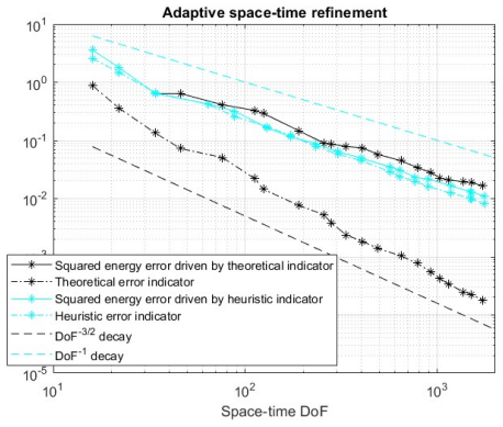
- For singular solutions, adaptive space-time BEM attains approximately twice the energy-norm convergence rate of uniform refinements: O(DoF^{-1}) versus O(DoF^{-1/2}) in the endpoint-singular example, and O(DoF^{-1/2}) versus roughly O(DoF^{-1/4}) for combined spatial/temporal singularities.
- At fixed accuracy, the adaptive method uses fewer degrees of freedom and, despite losing the block-Toeplitz structure of uniform time-stepping meshes, can consume less memory.
- The heuristic indicator, which weights only the spatial gradient by Δx_j, converges at the same rate as the energy error, while the rigorous indicator estimates a weaker norm.
- The approach is ready for extension to 3D scattering, where larger savings in DoFs and memory are expected, and to higher-order hp discretizations and nonlinear contact problems.
Reading between the lines
- Because the rigorous bound behind the indicator is stated for σ>0 but all experiments use σ=0, the certified reliability of the indicator in the computed regime remains an open point; a test of the ratio of true error to indicated error on refined meshes would settle whether the observed rates are also certified.
- The roughly doubled rates on singular problems echo the classical benefit of adaptive mesh refinement for elliptic problems; the paper's examples suggest the same benefit carries to hyperbolic space-time, but the theory of optimality for non-shape-regular or anisotropic space-time meshes is left open (the paper itself flags this).
- The success of the cheaper heuristic indicator hints that the full max-weight combination of gradients may be unnecessary in practice; a traveling-wave-front example in 3D could probe the limits of this simplification.
Editorial analysis
A structured set of objections, weighed in public.
Referee Report
Summary. The manuscript introduces a fully space-time adaptive boundary element method for the two-dimensional time-domain wave equation with Dirichlet boundary conditions. Starting from the energetic Galerkin formulation, the authors use residual-type local indicators motivated by the a posteriori bound in Theorem 3.1, perform Dörfler marking, and refine marked space-time elements by halving in both time and space. The main contribution is algorithmic: implementation of local tensor-product refinement, assembly and update of the non-Toeplitz Galerkin matrix, and numerical evaluation of the residual indicators. Four numerical experiments (smooth solution, localized peak, endpoint singularity, endpoint plus temporal singularity) are presented. For the singular examples, the measured energy-norm convergence rates on adaptively refined meshes are reported to be about twice those on uniform meshes, and memory savings are documented.
Significance. If the observed rate doubling is robust, this is the first systematic demonstration of fully space-time adaptive BEM for the 2D wave equation and a useful step toward 3D and nonlinear problems. The paper's strengths include the detailed algorithmic description, the honest separation between the rigorous a posteriori estimate and the heuristic indicator, and the breadth of numerical experiments. However, the central convergence-rate claims rest on Richardson-extrapolated benchmark energies computed from the same uniform Galerkin scheme, with no independent validation; in the singular cases the extrapolation is not in the asymptotic regime. The mismatch between the sigma>0 theory and the sigma=0 computations is also not addressed. With independent benchmarks and a sensitivity analysis, the conclusions could become convincing.
major comments (3)
- [§5.3, §5.4; Figs. 17 and 23] All energy errors in the singular examples are measured against benchmark values E≈2.07339e+01 (Example 5.3) and E≈3.64917 (Example 5.4), inferred by Richardson extrapolation from the same uniform Galerkin energies E^{(i)}_{Δt,Δx}. The quoted quotients are 3.3372 and 1.317, far from the value ≈4 observed in the smooth examples; this indicates that the sequence is not in the asymptotic regime, so the extrapolated benchmark can be systematically biased. Since the plotted quantity is the difference between E and the discrete energy, any bias changes the slopes of both the uniform and the adaptive curves and can produce a spurious factor of two in the rate ratio. The manuscript provides no independent reference (manufactured solution, higher-order discretization, or convolution quadrature) to validate these benchmarks. This is load-bearing for the central claim of approximately doubled conve
- [Remark, §2; Theorem 3.1, Eq. (13)] The residual bound (13) is stated with a constant depending on σ, and the cited theory in [23] is for fixed σ>0. All experiments set σ=0, justified only by the remark 'as usual'. No argument is supplied that the constant in (13) remains finite as σ→0, nor that the norm used in the plots is the correct limit. Consequently, the 'theoretical' indicators used for marking are not rigorously guaranteed to bound the error in the computed setting. Since the adaptive algorithm is advertised as based on a posteriori error estimates, this gap should be addressed at least by a limiting argument or by explicitly classifying the σ=0 indicator as heuristic.
- [§5.1 and §5.4] In Example 5.1 the exact solution ψ(t,x)=xt is known, and the exact energy could be computed directly, yet the benchmark is still obtained by Richardson extrapolation. This is a missed opportunity to validate the benchmark procedure against a ground truth. Conversely, in Example 5.4 the datum f(t,x)=H(t)t^{2/3} is not in H^2_σ(R+, H^{1/2}(Γ)) as required by Corollary 2.3, because its second time derivative is not square-integrable near t=0. The paper does not discuss whether the weak formulation and the a posteriori bound remain valid for such data. These two issues together weaken the evidence for the claimed rates in the singular cases.
minor comments (6)
- [Eq. (17)] The formula for β_i contains the undefined exponent 'γ+1'; presumably a typo.
- [Section 4.3] The function F is defined with a Heaviside factor H(t−τ) but the subsequent formula for ∂_tR would be clearer if the intended domain of the Heaviside factors were specified explicitly.
- [Section 6 vs Theorem 3.1] Section 6 attributes the residual estimate to [19], while Theorem 3.1 cites [23]. Please unify the references.
- [Example 5.2] The formula for f in the second branch appears to have a missing parenthesis: 'sin^4(4π(−t−2/8)' should likely read sin^4(4π(−t−2/8)) or similar.
- [Notation, Section 3] The norm ∥·∥_{0,0,S_j} is used without definition; please define it as the L^2(S_j) norm.
- [Figures 17 and 23] The slopes of the adaptive and uniform error curves would be easier to assess if each figure included a table of the fitted convergence rates and the range of DoFs used for the fit.
Circularity Check
Rate claims are partially self-referential because benchmark energies are Richardson-extrapolated from the same uniform Galerkin scheme; the core adaptive derivation itself is not circular.
-
fitted input called prediction
[Section 5.3 (benchmark inference, p.13); also Section 5.4 (p.16); energy defined in Eq. (20); comparisons in Figures 17 and 23.]
"Denoting by E^{(i)}_{Δt,Δx} the discrete energy obtained for Δx=Δt=1/(10·2^i), we find the empirical rate of convergence for i=1,2,3, (E^{(i+1)}_{Δt,Δx}-E^{(i)}_{Δt,Δx})/(E^{(i)}_{Δt,Δx}-E^{(i-1)}_{Δt,Δx}) ≃ 3.3372 and infer a benchmark value E≈2.07339e+01 for the exact energy."
The reference value E used to define every plotted 'squared energy error' is not an independent exact energy but a Richardson extrapolation from the same uniform Galerkin energies E^{(i)} (Section 5.4 repeats this with q≈1.317 and E≈3.64917). The uniform error sequence E−E^{(i)} is therefore the tail of the very sequence whose consecutive ratios define the empirical rate q; the uniform slope in Figures 17/23 is imposed by the extrapolation assumption rather than measured against a known solution. The paper itself says the uniform solution in Example 5.3 is 'still in a pre-asymptotic regime', so the extrapolated reference is not established. The claimed factor-of-two adaptive-vs-uniform improvement is a ratio of two curves sharing this same self-referential benchmark, so the improvement is
full rationale
The central derivation is not circular: Theorem 3.1 is quoted from prior published work [23] as an external a posteriori estimate, the indicators are evaluated from the actual Galerkin residual by quadrature, and the adaptive refinement loop does not use the benchmark energy as an input. The claim that adaptivity roughly doubles the uniform rate is an empirical observation, not a logical consequence of the definitions. However, two caveats matter. First, the 'exact' energies used to define energy errors are Richardson-extrapolated from the same uniform Galerkin family, so the uniform baseline rate is partly self-confirming and the adaptive comparison is not against an independent reference. Second, Theorem 3.1 is cited for σ>0 with constants depending on σ, while all computations set σ=0 (Section 2 Remark), so the theoretical reliability of the indicators in the computed regime is not established. These are correctness and validation risks rather than definitional reductions; [23] sharing an author (Gimperlein) is not itself circular, since it is an independent published theorem. Overall, the adaptive method's construction is not equivalent to its inputs, but the headline rate comparison is partly self-referential, justifying a moderate score.
Assumptions & free parameters
free parameters (2)
- Marking parameter Θ =
0.2 (Example 5.1), 0.5 (Examples 5.2–5.4)
- Benchmark exact energy E =
≈0.037135 (5.1), 35.7403 (5.2), 20.7339 (5.3), 3.64917 (5.4)
assumptions (4)
- standard math Theorem 2.1: continuity and weak coercivity of V and ∂_t V in anisotropic Sobolev spaces
- domain assumption Theorem 3.1: residual a posteriori error estimate (Eq. 13) bounding ||ψ−ψ_h|| by elementwise residual terms
- domain assumption Γ is a polygonal Lipschitz boundary or open polygonal Lipschitz curve; numerical experiments use the flat screen Γ=[0,1]×{0}
- ad hoc to paper Richardson extrapolation validity: the quotients (E_{i+1}−E_i)/(E_i−E_{i−1}) are assumed to converge to a constant, allowing inference of the 'exact' energy E
Cite this review
Pith. "Pith review of A space-time adaptive boundary element method for the wave equation." pith.science (2026). https://pith.science/paper/YADOQLWZ
@misc{pith2026251104265,
  author       = {Pith},
  title        = {Pith review of: A space-time adaptive boundary element method for the wave equation},
  year         = {2026},
  howpublished = {\url{https://pith.science/paper/YADOQLWZ}},
  note         = {Machine review of arXiv:2511.04265}
}
read the original abstract
This article initiates the study of space-time adaptive mesh refinements for time-dependent boundary element formulations of wave equations. Based on error indicators of residual type, we formulate an adaptive boundary element procedure for acoustic soft-scattering problems with local tensor-product refinements of the space-time mesh. We discuss the algorithmic challenges and investigate the proposed method in numerical experiments. In particular, we study the performance and improved convergence rates with respect to the energy norm for problems dominated by spatial, temporal or traveling singularities of the solution. The efficiency of the considered rigorous and heuristic a posteriori error indicators is discussed.
Figures


Figures from the paper (20 more)






Reference graph
Works this paper leans on
-
[19]
Gimperlein, F
H. Gimperlein, F. Meyer, D. Stark, C. \" O zdemir and E. P. Stephan , Boundary elements with mesh refinements for the wave equation , Numerische Mathematik, 139 (2018), pp. 867--912
2018
-
[23]
Gimperlein, C
H. Gimperlein, C. \" O zdemir, D. Stark, and E. P. Stephan , A residual a posteriori estimate for the time-domain boundary element method , Numerische Mathematik, 146 (2020), pp. 239--280
2020
-
[1]
A. Aimi, L. Desiderio, and G. Di Credico , Partially pivoted ACA based acceleration of the energetic BEM for time-domain acoustic and elastic waves exterior problems , Computers & Mathematics with Applications, 119 (2022), pp. 351--370
2022
-
[2]
A. Aimi, G. Di Credico, and H. Gimperlein , Time domain boundary elements for elastodynamic contact , Computer Methods in Applied Mechanics and Engineering, 415 (2023), p. 116296
2023
-
[3]
A. Aimi, G. Di Credico , H. Gimperlein, and C. Guardasoni , Adaptive time-domain boundary element methods for the wave equation with N eumann boundary conditions , Computers & Mathematics with Applications, 198 (2025), pp. 196--213
2025
-
[4]
A. Aimi, G. Di Credico, H. Gimperlein, and E. P. Stephan , Higher-order time domain boundary elements for elastodynamics: graded meshes and hp versions , Numerische Mathematik, 154 (2023), pp. 35--101
2023
-
[5]
A. Aimi, M. Diligenti, and C. Guardasoni , Numerical integration schemes for applications of energetic galerkin BEM to wave propagation problems , Rivista Matematica dell'Università di Parma, 2 (2011), pp. 147--187
2011
-
[6]
A. Aimi, M. Diligenti, C. Guardasoni, I. Mazzieri, and S. Panizzi , An energy approach to space-time G alerkin BEM for wave propagation problems , Internat. J. Numer. Methods Engrg., 80 (2009), pp. 1196--1240
2009
Show all 41 references
-
[7]
Bamberger and T
A. Bamberger and T. Ha Duong , Formulation variationnelle espace-temps pour le calcul par potentiel retardé de la diffraction d'une onde acoustique , Math. Meth. Appl. Sci., 8 (1986), pp. 405--435 and 598--608
1986
-
[8]
Banjai and F.-J
L. Banjai and F.-J. Sayas , Integral equation methods for evolutionary pde , Springer Ser. Comput. Math., Springer, Cham, (2022)
2022
-
[9]
Bertoluzza, S
S. Bertoluzza, S. Falletta, and L. Scuderi , Wavelets and convolution quadrature for the efficient solution of a 2d space-time BIE for the wave equation , Applied Mathematics and Computation, 366 (2020), p. 124726
2020
-
[10]
Bonito, C
A. Bonito, C. Canuto, R. H. Nochetto, and A. Veeser , Adaptive finite element methods , Acta Numerica, 33 (2024), pp. 163--485
2024
-
[11]
T. Chaumont-Frelet , Asymptotically constant-free and polynomial-degree-robust a posteriori estimates for space discretizations of the wave equation , SIAM Journal on Scientific Computing, 45 (2023), pp. A1591--A1620
2023
-
[12]
Chaumont-Frelet and A
T. Chaumont-Frelet and A. Ern , Damped energy-norm a posteriori error estimates using C 2-reconstructions for the fully discrete wave equation with the leapfrog scheme , ESAIM: Mathematical Modelling and Numerical Analysis, 59 (2025), pp. 1937--1972
2025
-
[13]
Cicci , Step control for the generalized convolution quadrature of the first order , M
L. Cicci , Step control for the generalized convolution quadrature of the first order , M . S c. thesis, University of Rome, 2017
2017
-
[14]
Costabel and F.-J
M. Costabel and F.-J. Sayas , Encyclopedia of Computational Mechanics, Second Edition , E. Stein, R. de Borst and J. R. Hughes, 2017, ch. Time-dependent problems with the boundary integral equation method, pp. 1--24
2017
-
[15]
Desiderio and S
L. Desiderio and S. Falletta , Efficient solution of two-dimensional wave propagation problems by CQ -wavelet BEM : algorithm and applications , SIAM Journal on Scientific Computing, 42 (2020), pp. B894--B920
2020
-
[16]
Dom \' nguez, T
V. Dom \' nguez, T. S \'a nchez-Vizuet, and F.-J. Sayas , A fully discrete C alder \'o n calculus for the two-dimensional elastic wave equation , Computers & Mathematics with Applications, 69 (2015), pp. 620--635
2015
-
[17]
Gantner and R
G. Gantner and R. van Veneti\" e , Adaptive space-time BEM for the heat equation , Computers & Mathematics with Applications, 107 (2022), pp. 117--131
2022
-
[18]
Gimperlein, M
H. Gimperlein, M. Maischak, and E. P. Stephan , Adaptive time domain boundary element methods with engineering applications , The Journal of Integral Equations and Applications, 29 (2017), pp. 75--105
2017
-
[20]
Gimperlein, F
H. Gimperlein, F. Meyer, C. \"O zdemir, and E. P. Stephan , Time domain boundary elements for dynamic contact problems , Computer Methods in Applied Mechanics and Engineering, 333 (2018), pp. 147--175
2018
-
[21]
Gimperlein, Z
H. Gimperlein, Z. Nezhi, and E. P. Stephan , A priori error estimates for a time-dependent boundary element method for the acoustic wave equation in a half-space , Mathematical Methods in the Applied Sciences, 40 (2017), pp. 448--462
2017
-
[22]
Gimperlein, C
H. Gimperlein, C. \"O zdemir, D. Stark, and E. P. Stephan , hp-version time domain boundary elements for the wave equation on quasi-uniform meshes , Computer Methods in Applied Mechanics and Engineering, 356 (2019), pp. 145--174
2019
-
[24]
Gimperlein and J
H. Gimperlein and J. Stocek , Space--time adaptive finite elements for nonlocal parabolic variational inequalities , Computer Methods in Applied Mechanics and Engineering, 352 (2019), pp. 137--171
2019
-
[25]
Glaefke , Adaptive Methods for Time Domain Boundary Integral Equations , PhD thesis, Brunel University, 2012
M. Glaefke , Adaptive Methods for Time Domain Boundary Integral Equations , PhD thesis, Brunel University, 2012
2012
-
[26]
Gwinner and E
J. Gwinner and E. P. Stephan , Advanced boundary element methods -- treatment of boundary value, transmission and contact problems , vol. 52 of Springer Series in Computational Mathematics, 2018
2018
-
[27]
Ha Duong , On retarded potential boundary integral equations and their discretizations , in Topics in computational wave propagation, Springer, ed., vol
T. Ha Duong , On retarded potential boundary integral equations and their discretizations , in Topics in computational wave propagation, Springer, ed., vol. 31 of Lect. Notes Comput. Sci. Eng., Berlin, 2003, p. 301–336
2003
-
[28]
Hoonhout, R
D. Hoonhout, R. Löscher, O. Steinbach, and C. Urzúa-Torres , Stable least-squares space-time boundary element methods for the wave equation . arxiv:2312.12547, 2023
2023 arXiv
-
[29]
Lopez-Fernandez and S
M. Lopez-Fernandez and S. Sauter , Generalized convolution quadrature with variable time stepping , IMA Journal of Numerical Analysis, 33 (2013), pp. 1156--1175
2013
-
[30]
Lopez-Fernandez and S
M. Lopez-Fernandez and S. Sauter , Generalized convolution quadrature with variable time stepping. part ii: Algorithm and numerical results , Applied Numerical Mathematics, 94 (2015), pp. 88--105
2015
-
[31]
A. B. Menon and M. Schanz , Adaptive time stepping for generalized convolution quadrature , PAMM, 23 (2023), p. e202300084
2023
-
[32]
M\" u ller and C
F. M\" u ller and C. Schwab , Finite elements with mesh refinement for wave equations in polygons , J. Comp. Appl. Math., 283 (2015), pp. 163--181
2015
-
[33]
P\" o lz and M
D. P\" o lz and M. Schanz , Space-time discretized retarded potential boundary integral operators: quadrature for collocation methods , SIAM Journal on Scientific Computing, 41 (2019), pp. A3860--A3886
2019
-
[34]
Pölz and M
D. Pölz and M. Schanz , On the space-time discretization of variational retarded potential boundary integral equations , Computers & Mathematics with Applications, 99 (2021), pp. 195--210
2021
-
[35]
Sauter and A
S. Sauter and A. Veit , Adaptive time discretization for retarded potentials , Numer. Math., 132 (2016), pp. 569--595
2016
-
[36]
Sayas , Retarded potentials and time domain boundary integral equations: A road map , vol
F.-J. Sayas , Retarded potentials and time domain boundary integral equations: A road map , vol. 50 of Springer Series in Computational Mathematics, 2016
2016
-
[37]
Steinbach and C
O. Steinbach and C. Urz\' u a-Torres , A new approach to space-time boundary integral equations for the wave equation , SIAM J. on Mathematical Analysis, 54 (2022), pp. 1370--1392
2022
-
[38]
A. Veit, M. Merta, J. Zapletal, and D. Lukas , Efficient solution of time-domain boundary integral equations arising in sound-hard scattering , Internat. J. Numer. Meth. Eng., 107 (2016), pp. 430--449
2016
-
[39]
Zank , Inf-sup stable space-time methods for time-dependent partial differential equations , Verlag der Technischen Universit \"a t Graz, 2020
M. Zank , Inf-sup stable space-time methods for time-dependent partial differential equations , Verlag der Technischen Universit \"a t Graz, 2020
2020
-
[40]
Zank and O
M. Zank and O. Steinbach , Adaptive space‐time boundary element methods for the wave equation , PAMM, 16 (2016), pp. 777--778
2016
-
[41]
O. C. Zienkiewicz and J. Z. Zhu , The superconvergent patch recovery and a posteriori error estimates. part 2: Error estimates and adaptivity , International Journal for Numerical Methods in Engineering, 33 (1992), pp. 1365--1382
1992
Reviewed August 3, 2026 · model on record in the stance chip above.
Discussion (0). Continue with ORCID to comment.