REVIEW 3 major objections 5 minor 30 references
Angular Resolution of Closely-Spaced Targets with Antenna Arrays
T0 review · 3 major / 5 minor · reviewed 2026-08-14 · deepseek-v4-flash
Pith's one-line read Maximum-likelihood resolution of closely spaced radar targets reduces to minimizing one residual-energy function, and a sequential test on the averaged residual counts the targets while holding the false-alarm probability at a chosen level.
desk verdict A clean translation of a 1982 ML superresolution dissertation that still reads well, but it is a historical document, not a new result, and its Type-1 error control is honestly conditional on noise-model knowledge. read the letter →
The pith
A machine-rendered reading of the paper's core claim, the machinery that carries it, and where it could break.
The reading
What carries the argument
The load-bearing object is the projection residual $Q(\omega) = z^*\Gamma(\omega)z$, where $\Gamma = I - A(\omega)(A(\omega)^*A(\omega))^{-1}A(\omega)^*$ is the orthogonal projector onto the orthogonal complement of the signal subspace spanned by the $M$ steering vectors; $Q$ is literally the residual energy after the best fit of the assumed target directions is removed. Four structural facts about this object carry the argument. Minimizing $Q$ over the directions is equivalent to maximum-likelihood estimation, and the Hessian of $Q$ at the minimum is the inverse of the direction block of the Fisher information matrix (Theorem 4.3-2), connecting resolution accuracy to the local shape of the $Q$-surface. Uniqueness of the global minimum reduces to the purely algebraic strong or weak $M$-regularity conditions on the element positions, which tell a designer whether a given array can resolve $M$ targets at all. After the estimates are good, the normalized statistic $(2/\sigma^2)K\bar Q$ is $\chi^2$-distributed with $K(2N-2M)$ degrees of freedom when exactly $M$ targets are present, so a chosen false-alarm probability $\alpha$ becomes a closed-form threshold. Under the alternative, $K\bar Q$ is an averaged positive-definite Hermitian form in complex Gaussian variables, and Theorem 7.2-2 gives its probability density in closed form, converting the threshold into detection probabilities.
What would settle it
Simulate the sequential multihypothesis test with no targets present: with known $\sigma^2 I$ noise, the empirical frequency of declaring one or more targets should sit at the chosen $\alpha$ up to the $\chi^2$-to-normal approximation the paper quotes for $N = 21$. The same simulation with the noise-model violations the paper tested, namely 1 dB per-channel power fluctuations or a sidelobe jammer of comparable power while the un-corrected threshold is used, should show the false-alarm rate and detection probability moving away from the predicted values, exactly the sensitivity documented in the paper's own figures.
Extended reading notes
Core claim
The paper's central claim is that resolving $M$ closely spaced point targets with an antenna array is a maximum-likelihood problem whose solution is the global minimum of a single scalar function: $Q(\omega) = z^*\Gamma(\omega)z$ with $\Gamma = I - A(A^*A)^{-1}A^*$, the squared residual of the data after its component in the span of the $M$ assumed steering vectors is removed. Minimizing $Q$ is exactly ML direction estimation, and Theorem 4.3-2 states that the second-derivative (curvature) matrix of $Q$ at the true minimum is the inverse of the direction block of the Fisher information matrix, so the accuracy of the estimate is governed by the curvature of this surface. Existence and uniqueness of the global minimum are guaranteed by the array geometry: a strongly $M$-regular layout, meaning every $2M$ steering vectors $a(\omega_1), \dots, a(\omega_{2M})$ are linearly independent (requiring $N \geq 2M$), suffices for a single spatial sample, while with several temporal samples and a regular covariance of the complex amplitudes, only weak $M$-regularity, meaning every $M+1$ steering vectors are independent (requiring $N \geq M+1$), is needed. For detection, the paper proves that the averaged statistic $\bar Q = \frac{1}{K} \sum_{k=1}^K \|\hat\Gamma z_k\|^2$ is the maximally invariant data reduction, that $(2/\sigma^2)K\bar Q$ is approximately $\chi^2$-distributed with $K(2N-2M)$ degrees of freedom under the hypothesis of $M$ targets, and that a sequential multihypothesis test built on this statistic keeps the probability of overestimating the number of targets near a prescribed level $\alpha$; detection probabilities are computed exactly for Swerling-II targets through the density of averaged positive-definite Hermitian forms (Theorem 7.2-2).
Load-bearing premise
The entire error-control machinery presumes that the noise is Gaussian with known covariance (normalized to $\sigma^2 I$ in the derivation, or with its first two moments known); the paper itself reports that deviations from the assumed noise model are the most critical influence on the test, and without accurate noise moments the claimed level $\alpha$ is not attained.
Editorial extensions
If this is right
- Two targets separated by half a beamwidth can be resolved in about 17 iterations of the stochastic approximation, with direction standard deviations near 0.04 beamwidths, provided the total SNR is on the order of 16–17 dB (slightly higher for in-phase than for quadrature targets).
- Temporal sampling can substitute for spatial sampling: with several pulses, an array need only be weakly $M$-regular (a 3-element linear array suffices for two targets), and pulse-to-pulse phase fluctuations wash out the in-phase and opposite-phase configurations that defeat single-pulse estimation.
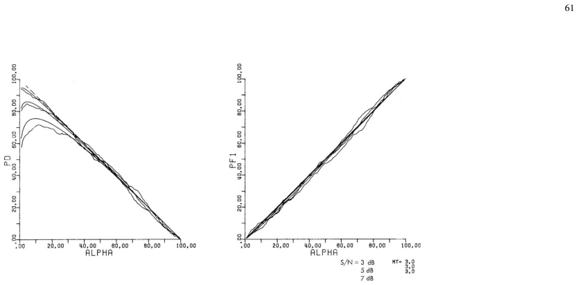
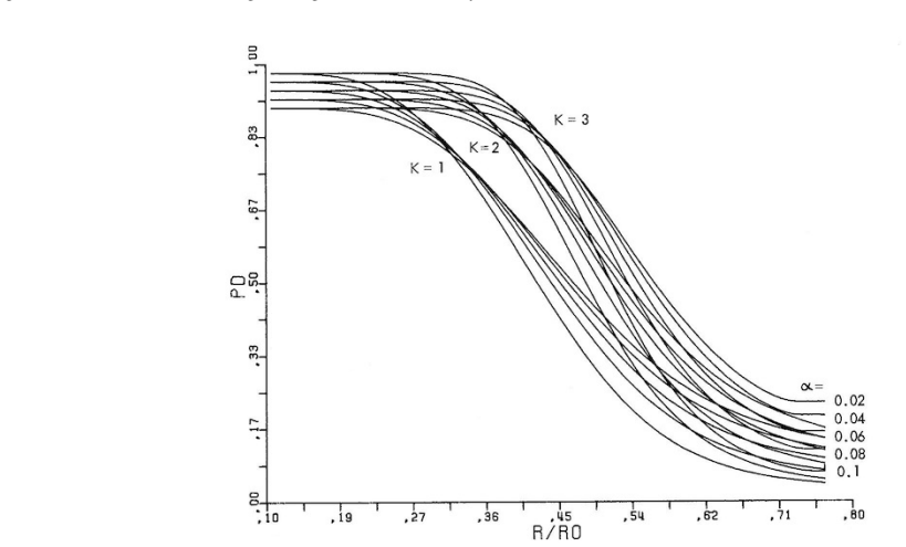
- The multihypothesis test holds the probability of overestimating the target count at the chosen level $\alpha$ (about 5–10% is recommended), and this control is essentially independent of the amplitude-fluctuation model; the Swerling-II detection curves serve as pessimistic lower bounds for the other models.
- The recursion is radar-friendly: each iteration consumes only the current sum-and-difference beam outputs, no data vector is stored, and for planar arrays the operation count favors the stochastic approximation over an averaged grid search.
- Single-pulse superresolution is not practical for radar, since it demands SNR above roughly 25 dB; the intended mode of use is the multi-pulse sequential procedure.
Reading between the lines
- The threshold formula $\eta = \sigma^2(\sqrt{(N-M)/K}\, U_\alpha + N-M)$ depends on no nuisance parameters besides the noise power $\sigma^2$, so the same test could be applied to spectral-line counting in time-sampled data, a transfer the introduction mentions but the paper does not develop, by estimating $\sigma^2$ from the residual at the largest fitted $M$.
- The paper's sensitivity results suggest a concrete extension it does not test: whiten the data with an estimated noise covariance and then apply the unchanged $\chi^2$ threshold; if the noise moments are recovered well, the nominal $\alpha$ should be restored in the correlated-noise cases where the paper's own simulations show it fails.
- The invariance of $Q$ under common element responses implies a design rule the paper stops short of stating: arrays built from matched subarrays with equal phase centers preserve the resolution test exactly, not merely approximately.
- The summary's direction-frequency ambiguity relation is qualitative; applying the same $Q$-curvature analysis to the time-sampled spectral-line formulation would make the trade-off quantitative and check whether the Cramér–Rao equivalence of Theorem 4.3-2 carries over to frequency estimation.
Signed reviews
Editorial analysis
A structured set of objections, weighed in public.
Referee Report
Summary. The manuscript, an authorized translation of Ulrich Nickel's 1982 doctoral dissertation, addresses maximum-likelihood angular superresolution of closely spaced far-field point targets and the estimation of the number of targets present. It derives the criterion Q(ω)=z*Γz from the Gaussian likelihood, introduces strong and weak M-regularity conditions for identifiability and uniqueness, characterizes estimation accuracy through the curvature of Q and the Cramér-Rao bound, proposes a Robbins-Monro stochastic-approximation algorithm using sum and difference beams, and constructs a sequential multihypothesis test based on the averaged statistic Q̄ with a chi-square/normal threshold. Analytic detection probabilities for Swerling-II targets are derived via the distribution of averaged Hermitian forms, and extensive simulations examine robustness to coupling, extended targets, quantization, and noise mismatch.
Significance. If the results hold, the paper is a rigorous early treatment of ML superresolution and model-order selection, and several elements remain valuable: the Q-function formulation, the CRLB-based resolution curves, the stochastic-approximation implementation, and the closed-form detection probabilities of Theorem 7.2-2. The appendices contain complete proofs of the principal theorems and careful moment calculations, and the analytic detection formula is a parameter-free prediction in terms of the eigenvalues of A*ΓAB and σ², tested by simulation. The principal limitation, acknowledged in the text, is that the Type-1 error control of the sequential test is approximate and depends on exact knowledge of the noise covariance and on asymptotic convergence; the simulations show degradation under 1-dB noise mismatch and jamming. With these conditions made explicit, the paper is a useful archival contribution.
major comments (3)
- [§7.1, Eqs. (7.1-3)–(7.1-6); §7.3, Figs. 7-4/7-5] The claimed approximate Type-1 error control of the sequential test rests on the approximations Γ̂Ab_i≈0 (7.1-3) and exactly known σ²I noise, and the convergence supporting the first approximation is only asymptotic (Corollary 5.1-8). The operating regime of Chapter 7 (17 iterations, K=2–4 samples, SNR 3–7 dB) is finite, and no bound on ‖Γ̂Ab_i‖ is provided for that regime. The paper's own simulations show that 1-dB receiver-noise fluctuations make the test miss level α and that an unmodeled jammer roughly halves the detection probability (Figs. 7-4, 7-5; Summary item 9). The headline claim should be restated as conditional on exact noise moments and sufficiently converged estimates; as written it is stronger than what is proved.
- [§5.1, Eq. (5.1-7) and Corollary (5.1-8)] The Ljung theorem requires that all trajectories of ˙ω=−grad E{Q} starting in Ω2 remain in Ω1, and the text states that this cannot generally be verified because the location of the minimum in Ω1 is unknown. The assertion that 'all considered cuts' show M(ωg) to be part of the attraction region is an empirical statement, not a proof. Since convergence of the stochastic approximation is the estimation step on which the subsequent test relies, this missing verification is load-bearing; the paper should either prove the attraction-region condition for the arrays used or explicitly present the convergence result as conditional on the Ljung hypotheses, with the simulations as supporting evidence.
- [§3.3, Eq. (3.3-3); §7.2 and §7.3] The factorization of the total error probability assumes independence of the individual tests ϕi, which the text itself says requires new data for each test. The implementation in Chapter 7 does not state clearly whether the Q̄_M statistics for different M are computed from independent K-sample sets or from the same data; if they are computed from the same data, the product formula (3.3-3) does not apply and no alternative bound is given. Please clarify the data-reuse policy and, if data are reused, provide an analysis of the dependence or a conservative bound.
minor comments (5)
- [Eq. (3.2-3)] The definition of Γ omits the inverse on (A*R^{-1}A); compare with the correct form in Eq. (3.2-1). This should be corrected.
- [Symbol list and §4.4] Several typographical and OCR artifacts remain in the translation, e.g., 'maping' in the symbol list, 'Kroneker' for 'Kronecker', and 'fiior' in §4.4; a thorough proofreading pass is needed.
- [§5.2, Figs. 5-6 to 5-9] The figure captions in the provided text are minimal and do not always identify which of the four correction-vector variants, which SNR, and which target model are plotted; adding complete captions would improve reproducibility.
- [§7.1, Eq. (7.1-5)] The normal approximation to the chi-square variable should state explicitly the range of N and K for which it is intended; the simulations use N=21 and K=2–4, and the text notes that the approximation is already 'sufficiently accurate' there, but no quantitative criterion is given.
- [§7.3, paragraph before Eq. (7.2-5)] The text refers to '(7.2-5)' for the unequal-noise moments, but the displayed formulas for E_n{Q̄} and var_n{Q̄} are not numbered in the manuscript; the equations should be labeled.
Circularity Check
Derivation is self-contained: Q-minimization and detection thresholds follow from the stated Gaussian model with no fitted parameter renamed as a prediction.
full rationale
No significant circularity is present. The central estimation result, minimization of Q(ω)=z*[I−A(A*A)^−1A*]z, is obtained by algebraically eliminating the complex amplitudes b from the Gaussian likelihood (Secs. 3.2 and 4.1), so it is a derived consequence of the model rather than an input. The uniqueness theorems (4.2-2 and 5.1-2) are proved directly from the stated strong/weak M-regularity assumptions using linear independence of the array manifold, with proofs included in the text and appendices. The accuracy claims are benchmarked against the Cramér-Rao lower bound, which is an external information-theoretic standard, not a fitted quantity. The multihypothesis test threshold η in (7.1-4)/(7.1-6) is derived from an explicitly stated approximation, Γ̂Ab≈0, which makes KQ̄ approximately chi-squared or normal under the assumed known noise covariance; the paper then validates this threshold by simulation. The paper itself flags in Sec. 7.3 and Summary item 9 that deviations from the noise model are the most critical limitation and shows in Figs. 7-4/7-5 that the claimed level α fails under 1-dB noise mismatch. This is an honest conditional claim with exposed assumptions, not circular reasoning: the guarantee is stated for the model in which it is derived, and its failure outside that model confirms it is a substantive prediction. The heuristic constants μ and η are tuned by simulation (Secs. 5.1, 5.2), but they affect convergence speed and correction-vector damping rather than the identifiability, CRLB, or Type-1 error claims, and they are not presented as derived predictions. External mathematical results cited, such as Ljung's stochastic-approximation theorem, Fabian's asymptotic-normality theorem, and Goodman's distribution theory, are standard independent results, not self-citations carrying the argument. No step in the paper reduces, by construction or by self-citation, to its own output.
Assumptions & free parameters
free parameters (2)
- Stochastic-approximation step-size coefficient mu =
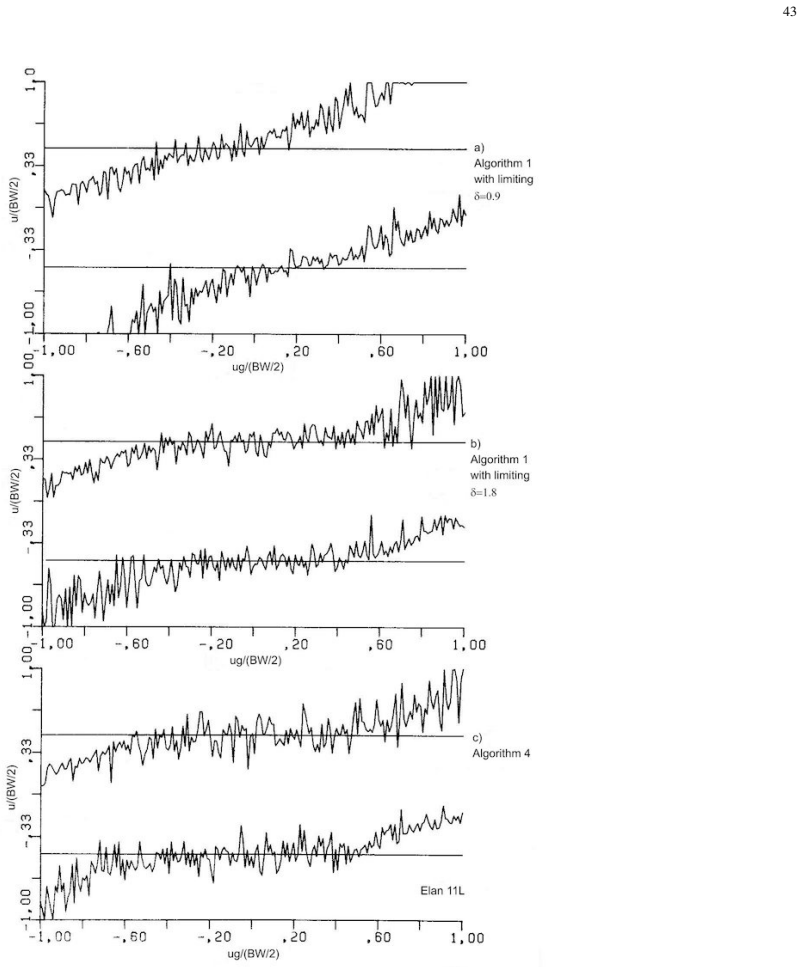
mu = delta/(ae) * BW/2 with delta=0.9 for linear arrays, delta=1.8 for planar arrays
- Correction-vector saturation bound eta =
eta = 0.8 * ae
assumptions (6)
- domain assumption Far-field point-target plane-wave signal model z = Ab + n with additive Gaussian noise, where targets are infinitely distant point scatterers (Eq. 2.1-1, 2.1-2).
- domain assumption The receiver noise is independent, zero-mean complex Gaussian with known covariance, normalized to a multiple of the identity for the main derivation (Section 2.2, and normalization sigma^2=1).
- domain assumption Array layouts satisfy strong M-regularity (4.2-1) or weak M-regularity (5.1-1) in the search region.
- standard math Ljung's theorem on recursive stochastic algorithms (Theorem 5.1-6) applies; the paper checks conditions including Lipschitz continuity and the existence of fourth moments.
- domain assumption After a good estimate, the residual projection satisfies Gamma Ab approximately 0, making Q_bar approximately chi-squared distributed with 2(N-M)K degrees of freedom (Eq. 7.1-3).
- domain assumption Ergodic averaging: time averages of zz* and bb* converge to expected values, so K-sample ML minimization is replaced by expected Q (Eq. 3.2-4).
Cite this review
Pith. "Pith review of Angular Resolution of Closely-Spaced Targets with Antenna Arrays." pith.science (2026). https://pith.science/paper/YEOL7LCF
@misc{pith2026190805308,
  author       = {Pith},
  title        = {Pith review of: Angular Resolution of Closely-Spaced Targets with Antenna Arrays},
  year         = {2026},
  howpublished = {\url{https://pith.science/paper/YEOL7LCF}},
  note         = {Machine review of arXiv:1908.05308}
}
read the original abstract
This is an English translation of Ulrich Nickel's PhD dissertation with the original title "Winkelaufl\"osung eng benachbarter Ziele mit Gruppenantennen." It describes maximum-likelihood angular superresolution of closely-spaced targets. It also discusses estimating the number of targets present.
Figures


Figures from the paper (42 more)








Reference graph
Works this paper leans on
-
[1]
M. I. Skolnik, Radar Handbook. McGraw Hill, 1970
work page 1970
-
[2]
Über eine Klassifizierungsmöglichkeit von Radarzielen mittels kohärent gemessener Echosignale,
K. von Schlachta, “Über eine Klassifizierungsmöglichkeit von Radarzielen mittels kohärent gemessener Echosignale,” Ph.D. dissertation, TU Berlin, 1977
work page 1977
-
[3]
Generalized likelihood signal resolution,
J. A. Stuller, “Generalized likelihood signal resolution,” IEEE Trans. IT , vol. 21, no. 3, May 1975
work page 1975
-
[4]
H. Witting and G. Nölle, Angewandte mathematische Statistik . Stuttgart: Teubner, 1970
work page 1970
-
[5]
N. R. Goodman, “Statistical analysis based on a certain multivariate complex gaussian distribution (an introduction),” Ann. of Math. Stat. , vol. 34, 1963
work page 1963
-
[6]
Analysis of recursive stochastic algorithms,
L. Ljung, “Analysis of recursive stochastic algorithms,” IEEE Transactions on Automatic Control , vol. 22, no. 4, Aug. 1977
work page 1977
-
[7]
Data adaptive spectral analysis,
R. T. Lacoss, “Data adaptive spectral analysis,” Geophysics, vol. 36, pp. 661–675, Aug. 1971
work page 1971
-
[8]
Maximum entropy spectral analysis and autoregressive decomposition,
T. J. Ulrych and T. N. Bishop, “Maximum entropy spectral analysis and autoregressive decomposition,” Rev. Geophysics and Space Phys. , vol. 13, pp. 183–200, Feb. 1975
work page 1975
Show all 30 references
-
[9]
Optimum space-time signal processing and parameter estimation,
G. O. Young, “Optimum space-time signal processing and parameter estimation,” IEEE Transactions on Aerospace and Electronic Systems , vol. 4, no. 3, May 1968
1968
-
[10]
Applications of space-time decision and estimation theory to antenna processing system-design,
G. O. Young and J. E. Howard, “Applications of space-time decision and estimation theory to antenna processing system-design,” Proceedings of the IEEE, vol. 38, no. 5, May 1970
1970
-
[11]
A decision theoretic approach to the angular resolution and parameter estimation of multiple targets,
A. A. Ksienki and R. B. McGhee, “A decision theoretic approach to the angular resolution and parameter estimation of multiple targets,”IEEE Transactions on Aerospace and Electronic Systems , vol. 4, no. 3, May 1968
1968
-
[12]
Entdeckung und Parameterschätzung bei Zielen mit geringem Winkelabstand,
W. D. Wirth, “Entdeckung und Parameterschätzung bei Zielen mit geringem Winkelabstand,” FFM, Tech. Rep. 192, Oct. 1972
1972
-
[13]
Low-angle radar tracking in the presence of multipath,
W. D. White, “Low-angle radar tracking in the presence of multipath,” IEEE Transactions on Aerospace and Electronic Systems , vol. 10, no. 6, Nov. 1974
1974
-
[14]
Angular tracking of two closely spaced radar targets,
G. E. Pollon and G. W. Lank, “Angular tracking of two closely spaced radar targets,” IEEE Transactions on Aerospace and Electronic Systems , vol. 4, no. 4, Jul. 1968
1968
-
[15]
Array aperture sampling technique for multipath compensation,
F. G. Willwerth and I. Kupiec, “Array aperture sampling technique for multipath compensation,” Microwave Journal, Jun. 1976
1976
-
[16]
Direkt-lösende Algorithmen für die Interferenzanalyse Teil I und II,
K. Bauer, “Direkt-lösende Algorithmen für die Interferenzanalyse Teil I und II,” Frequenz, vol. 30, no. 4 and 5, 1976
1976
-
[17]
Multiple tone parameter estimation from discrete-time observations,
D. C. Rife and R. R. Boorstyn, “Multiple tone parameter estimation from discrete-time observations,” Bell Syst. Techn. J. , vol. 55, no. 9, Nov. 1976
1976
-
[18]
Signal processing techniques for resolving individual pulses in a multipath signal,
J. E. Ehrenberg, T. E. Ewart, and R. D. Morris, “Signal processing techniques for resolving individual pulses in a multipath signal,” J. Acoust. Soc. Am. , vol. 63, no. 6, Jun. 1978
1978
-
[19]
Maximum likelihood estimation of the number, directions, and strengths of point radio sources from variable baseline interferometer data,
I. N. El Behery and R. H. McPhie, “Maximum likelihood estimation of the number, directions, and strengths of point radio sources from variable baseline interferometer data,” IEEE Trans. AP , vol. 26, no. 2, Mar. 1978
1978
-
[20]
Parameter estimation of multiple signals,
R. A. Birgenheier, “Parameter estimation of multiple signals,” Ph.D. dissertation, University of California, Los Angeles, 1972
1972
-
[21]
T. W. Anderson, An introduction to Multivariate Statistical Analysis . J. Wiley, 1958
1958
-
[22]
Klingenberg, Eine Vorlesung über Differentialgeometrie
W. Klingenberg, Eine Vorlesung über Differentialgeometrie . Heidelberger Taschenbücher, Springer, 1973
1973
-
[23]
Riemannsche Geometrie im Großen,
D. Gromoll, W. Klingenberg, and W. Meyer, “Riemannsche Geometrie im Großen,” Lecture Notes in mathematics , vol. 55, 1975
1975
-
[24]
M. T. Wasan, Stochastic Approximation. Cambridge University Press, 1969
1969
-
[25]
Multiple Gaussian targets: the track-on-jam problem,
I. Kanter, “Multiple Gaussian targets: the track-on-jam problem,” IEEE Transactions on Aerospace and Electronic Systems , vol. 13, no. 6, Nov. 1977
1977
-
[26]
The ratio of functions of random variables,
——, “The ratio of functions of random variables,” IEEE Transactions on Aerospace and Electronic Systems , vol. 13, no. 6, Nov. 1977
1977
-
[27]
Robust estimation via stochastic approximation,
R. D. Martin and C. J. Masreliez, “Robust estimation via stochastic approximation,” IEEE Transactions on Information Theory , vol. 21, no. 3, May 1975
1975
-
[28]
Ein rechnergesteuertes Nahfeldvermessungsverfahren für elektronisch steuerbare Gruppenantennen,
G. Hüschelrath, “Ein rechnergesteuertes Nahfeldvermessungsverfahren für elektronisch steuerbare Gruppenantennen,” Ph.D. dissertation, TH Aachen, Feb. 1978
1978
-
[29]
Sum of exponential random variables,
J. C. Demaret and A. Garcet, “Sum of exponential random variables,” AEÜ, vol. 31, no. 11, 1977
1977
-
[30]
Stoer, Einführung in die Numerische Mathematik I
J. Stoer, Einführung in die Numerische Mathematik I . Springer, 1973
1973
Reviewed August 14, 2026 · model on record in the stance chip above.
Discussion (0). Continue with ORCID to comment.