Mapping climate change awareness through spatial hierarchical clustering
Pith reviewed 2026-05-23 21:02 UTC · model grok-4.3
The pith
Adding physical distances between countries to clustering yields more stable and compact groups by climate awareness.
A machine-rendered reading of the paper's core claim, the machinery that carries it, and where it could break.
Core claim
By combining climate change awareness measures, socio-economic factors, climate-related characteristics, and physical distances in a Ward-like hierarchical clustering algorithm, and using a customized hyperparameter selection that compares geographical and non-geographical partitions, the analysis identifies more stable, interpretable, and geographically-compact country groups, highlighting high awareness in Western countries versus lower awareness elsewhere.
What carries the argument
Geographically-informed Ward-like hierarchical clustering algorithm that incorporates physical distances alongside awareness and socio-economic features.
If this is right
- The geographically-informed partitions exhibit greater stability than those based solely on awareness and socio-economic data.
- Western countries form one high-awareness and geographically compact cluster.
- Asian, African, and Middle Eastern countries form groups with greater variability but overall lower awareness.
- The spatial component produces aggregations that are easier to interpret because they respect physical proximity.
Where Pith is reading between the lines
- The identified clusters could support region-specific strategies for raising climate awareness.
- The same spatial clustering approach might be tested on other cross-country attitude datasets such as public health or economic policy views.
- Re-running the analysis on newer awareness surveys would show whether the Western versus other-regions contrast persists over time.
Load-bearing premise
The climate change awareness measures, socio-economic indicators, and climate characteristics are accurate, comparable across countries, and relevant without systematic measurement error or selection bias.
What would settle it
Running the same data through a non-geographical clustering and finding equal or greater stability in the partitions, or obtaining awareness groups that shift markedly when independent survey data replace the current measures.
Figures









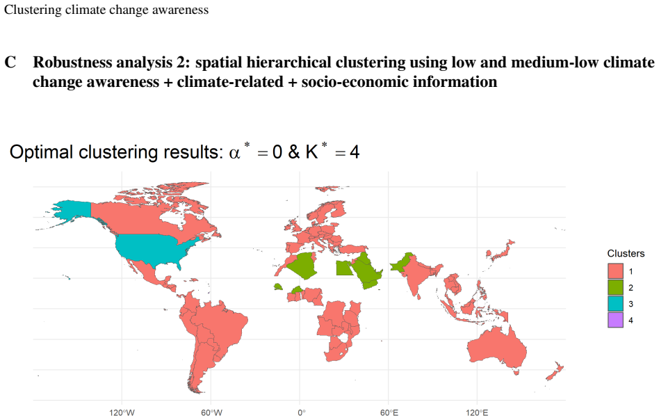
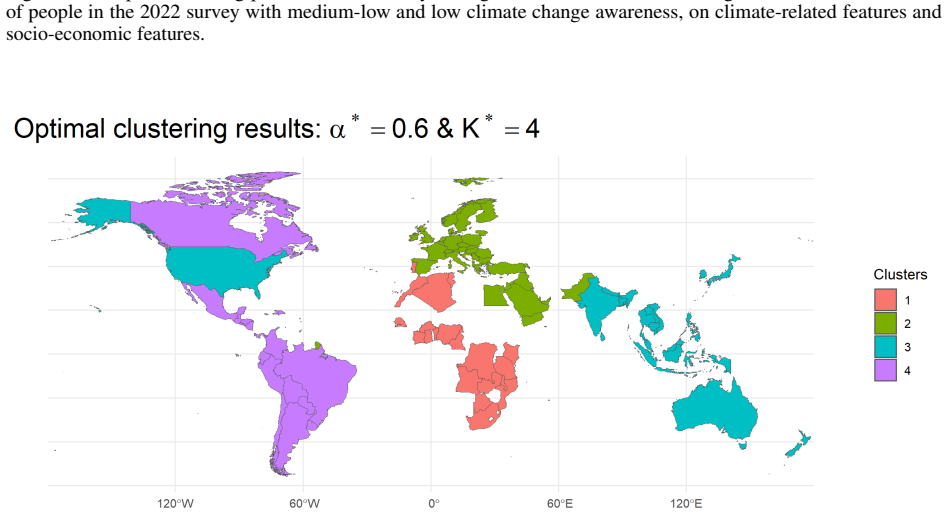


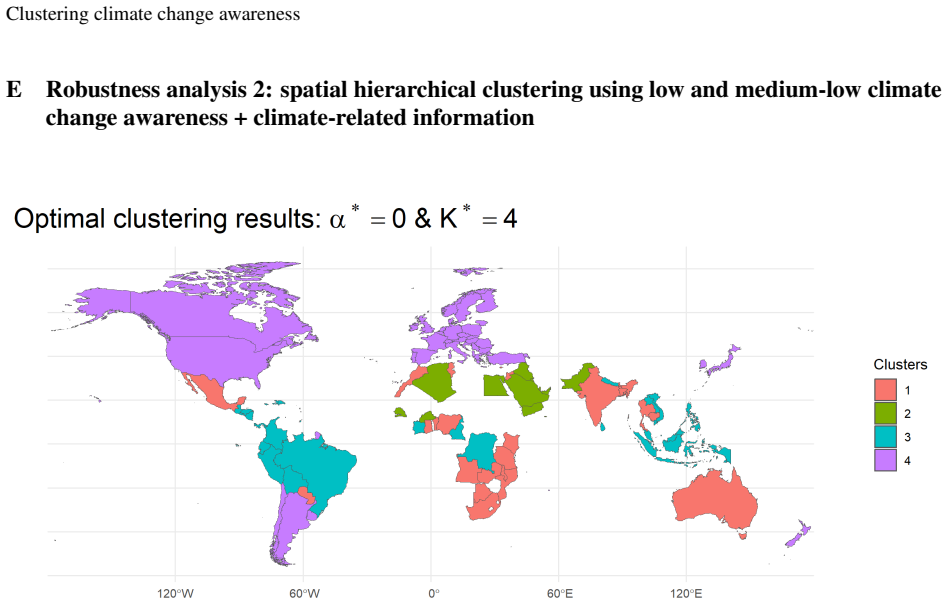


read the original abstract
Climate change is a critical issue that will be in the political agenda for the next decades. While it is important for this topic to be discussed at higher levels, it is also of paramount importance that the populations became aware of the problem. As different countries may face more or less severe repercussions, it is also useful to understand the degree of awareness of specific populations. In this paper, we present a geographically-informed hierarchical clustering analysis aimed at identify groups of countries with a similar level of climate change awareness. We employ a Ward-like clustering algorithm that combines information pertaining climate change awareness, socio-economic factors, climate-related characteristics of different countries, and the physical distances between countries. To choose suitable values for the clustering hyperparameters, we propose a customized algorithm that takes into account the within-clusters homogeneity, the between-clusters separation and that explicitly compares the geographically-informed and non-geographical partitioning. The results show that the geographically-informed clustering provides more stability of the partitions and leads to interpretable and geographically-compact aggregations compared to a clustering in which the geographical component is absent. In particular, we identify a clear contrast among Western countries, characterized by high and compact awareness, and Asian, African, and Middle Eastern countries having greater variability but still lower awareness.
Editorial analysis
A structured set of objections, weighed in public.
Referee Report
Summary. The paper claims that a geographically-informed hierarchical clustering (Ward-like algorithm incorporating climate awareness, socio-economic factors, climate characteristics, and physical distances) yields more stable partitions and geographically compact, interpretable country groups than a non-geographical version. A custom hyperparameter algorithm evaluates within-cluster homogeneity, between-cluster separation, and explicitly compares the two variants; results highlight a contrast between high-awareness Western countries and lower-awareness Asian/African/Middle Eastern ones.
Significance. If the stability and compactness advantages can be shown to hold under independent hyperparameter selection, the approach would offer a practical tool for identifying awareness patterns using external country-level data and a standard clustering objective. The explicit comparison of geo vs. non-geo variants is a methodological strength when properly validated, but the current lack of quantitative metrics reduces the immediate utility for policy or further research.
major comments (1)
- [Abstract and Methods] Abstract and Methods (description of customized hyperparameter algorithm): the procedure selects the number of clusters and distance weighting by explicitly comparing geo-informed and non-geographical partitions on homogeneity/separation criteria. This makes the reported gains in stability potentially circular, as the selection itself favors the geo variant; the manuscript must demonstrate the stability advantage with hyperparameters chosen independently (e.g., via a fixed criterion or separate validation set) rather than through the same comparison used to assert superiority.
minor comments (2)
- [Abstract] Abstract: no source, sample size, or quantitative stability metric (e.g., adjusted Rand index or silhouette score) is provided for the awareness data or the stability claim.
- [Results] Results: the final values chosen for the number of clusters and the geographical weighting parameter are not stated explicitly.
Simulated Author's Rebuttal
We thank the referee for highlighting a methodological concern regarding potential circularity in our hyperparameter selection. We agree this requires clarification and revision to strengthen the validity of our stability comparisons.
read point-by-point responses
-
Referee: [Abstract and Methods] Abstract and Methods (description of customized hyperparameter algorithm): the procedure selects the number of clusters and distance weighting by explicitly comparing geo-informed and non-geographical partitions on homogeneity/separation criteria. This makes the reported gains in stability potentially circular, as the selection itself favors the geo variant; the manuscript must demonstrate the stability advantage with hyperparameters chosen independently (e.g., via a fixed criterion or separate validation set) rather than through the same comparison used to assert superiority.
Authors: We acknowledge the validity of this concern: the customized algorithm's explicit comparison during selection could bias the reported stability advantages toward the geo-informed variant. In the revised manuscript, we will modify the Methods section to select the number of clusters (k) and geographic distance weighting using an independent, standard criterion (e.g., silhouette score or elbow method based on within-cluster homogeneity) applied separately to the geo-informed and non-geographical variants, without any cross-comparison in the selection step. Stability metrics (e.g., adjusted Rand index on bootstrap resamples) will then be computed and compared post-selection. The abstract, results, and discussion will be updated to describe this revised procedure and present the corresponding findings. This change ensures the stability evaluation is non-circular while preserving the core contribution of comparing the two clustering approaches. revision: yes
Circularity Check
Hyperparameter tuning explicitly compares geo vs non-geo partitions, making stability/compactness superiority claim reduce to the selection procedure
specific steps
-
fitted input called prediction
[Abstract]
"To choose suitable values for the clustering hyperparameters, we propose a customized algorithm that takes into account the within-clusters homogeneity, the between-clusters separation and that explicitly compares the geographically-informed and non-geographical partitioning. The results show that the geographically-informed clustering provides more stability of the partitions and leads to interpretable and geographically-compact aggregations compared to a clustering in which the geographical component is absent."
The hyperparameter selection procedure is defined to include an explicit geo vs non-geo comparison plus homogeneity/separation metrics; the paper then presents the outcome of that tuned comparison as evidence that geo-informed clustering is superior in stability and compactness. The claimed advantage is therefore generated by the same procedure used to select the model, rather than evaluated independently.
full rationale
The paper's central claim of geo-informed superiority rests on a customized hyperparameter algorithm whose selection criterion itself performs the geo vs non-geo comparison and homogeneity/separation evaluation. Because the tuning procedure incorporates the exact contrast later asserted as an independent result, the reported gains in stability and geographic compactness are not shown to be independent of the fitting process. No separate held-out validation or fixed-hyperparameter comparison is described. This matches the fitted-input-called-prediction pattern but is only partial because external data and standard clustering still supply the raw inputs.
Axiom & Free-Parameter Ledger
free parameters (1)
- clustering hyperparameters (number of clusters, weighting of distance term)
axioms (2)
- domain assumption Ward-like linkage combined with geographic distances yields stable and interpretable partitions of awareness data.
- domain assumption The awareness, socio-economic, and climate variables are measured without systematic cross-country bias.
Reference graph
Works this paper leans on
-
[1]
The velocity of climate change
Scott R Loarie, Philip B Duffy, Healy Hamilton, Gregory P Asner, Christopher B Field, and David D Ackerly. The velocity of climate change. Nature, 462(7276):1052–1055, 2009
work page 2009
-
[2]
Climate change: Strategies for mitigation and adaptation
Fang Wang, Jean Damascene Harindintwali, Ke Wei, Yuli Shan, Zhifu Mi, Mark John Costello, Sabine Grunwald, Zhaozhong Feng, Faming Wang, Yuming Guo, et al. Climate change: Strategies for mitigation and adaptation. The Innovation Geoscience, 1(1):100015–61, 2023
work page 2023
-
[3]
Multi-decadal increase of forest burned area in australia is linked to climate change
Josep G Canadell, CP Meyer, Garry D Cook, Andrew Dowdy, Peter R Briggs, Jürgen Knauer, Acacia Pepler, and Vanessa Haverd. Multi-decadal increase of forest burned area in australia is linked to climate change. Nature communications, 12(1):6921, 2021
work page 2021
-
[4]
Climate change is increasing the likelihood of extreme autumn wildfire conditions across california
Michael Goss, Daniel L Swain, John T Abatzoglou, Ali Sarhadi, Crystal A Kolden, A Park Williams, and Noah S Diffenbaugh. Climate change is increasing the likelihood of extreme autumn wildfire conditions across california. Environmental Research Letters, 15(9):094016, 2020
work page 2020
-
[5]
Understanding human influence on climate change in china
Ying Sun, Xuebin Zhang, Yihui Ding, Deliang Chen, Dahe Qin, and Panmao Zhai. Understanding human influence on climate change in china. National science review, 9(3):nwab113, 2022
work page 2022
-
[6]
Isabel Meza, Ehsan Eyshi Rezaei, Stefan Siebert, Gohar Ghazaryan, Hamideh Nouri, Olena Dubovyk, Helena Gerdener, Claudia Herbert, Jürgen Kusche, Eklavyya Popat, et al. Drought risk for agricultural systems in south africa: Drivers, spatial patterns, and implications for drought risk management. Science of the Total Environment, 799:149505, 2021
work page 2021
-
[7]
Recent responses to climate change reveal the drivers of species extinction and survival
Cristian Román-Palacios and John J Wiens. Recent responses to climate change reveal the drivers of species extinction and survival. Proceedings of the National Academy of Sciences, 117(8):4211–4217, 2020
work page 2020
-
[8]
A million threatened species? thirteen questions and answers, 2019
Purvis Andy. A million threatened species? thirteen questions and answers, 2019. https://www.ipbes.net/ news/million-threatened-species-thirteen-questions-answers , Last accessed on August 31 2024
work page 2019
-
[9]
Greenhouse effect, sea level rise, and coastal zone management
James G Titus. Greenhouse effect, sea level rise, and coastal zone management. Coastal Management, 14(3):147– 171, 1986
work page 1986
-
[10]
Sammy Zahran, Eunyi Kim, Xi Chen, and Mark Lubell. Ecological development and global climate change: A cross-national study of kyoto protocol ratification. Society and Natural Resources, 20(1):37–55, 2007
work page 2007
-
[11]
What are the costs of limiting co2 concentrations
James A Edmonds and Ronald D Sands. What are the costs of limiting co2 concentrations. Global climate change: The science, economics, and politics, pages 140–86, 2003
work page 2003
-
[12]
Global climate risk index, 2021
David Eckstein, Vera Künzel, and Schäfer Laura. Global climate risk index, 2021. https://reliefweb.int/ report/world/global-climate-risk-index-2021 , Last accessed on August 31 2024
work page 2021
-
[13]
A survey of constrained classification
AD Gordon. A survey of constrained classification. Computational Statistics & Data Analysis, 21(1):17–29, 1996
work page 1996
-
[14]
Clustering of spatial data by the em algorithm
Christophe Ambroise, Mo Dang, and Gérard Govaert. Clustering of spatial data by the em algorithm. In geoENV I—Geostatistics for Environmental Applications: Proceedings of the Geostatistics for Environmental Applications Workshop, Lisbon, Portugal, 18–19 November 1996, pages 493–504. Springer, 1997. 17 Clustering climate change awareness
work page 1996
-
[15]
Clustering spatial data with a geographic constraint: exploring local search
Zhung-Xun Liao and Wen-Chih Peng. Clustering spatial data with a geographic constraint: exploring local search. Knowledge and information systems, 31:153–170, 2012
work page 2012
-
[16]
Spatially constrained clustering of ecological networks
Vincent Miele, Franck Picard, and Stéphane Dray. Spatially constrained clustering of ecological networks. Methods in Ecology and Evolution, 5(8):771–779, 2014
work page 2014
-
[17]
Constrained clustering of irregularly sampled spatial data
Yudi Pawitan and Jian Huang. Constrained clustering of irregularly sampled spatial data. Journal of Statistical Computation and Simulation, 73(12):853–865, 2003
work page 2003
-
[18]
A geostatistical basis for spatial weighting in multivariate classification
MA Oliver and R Webster. A geostatistical basis for spatial weighting in multivariate classification. Mathematical geology, 21:15–35, 1989
work page 1989
-
[19]
The multivariate (co) variogram as a spatial weighting function in classification methods
Gilles Bourgault, Denis Marcotte, and Pierre Legendre. The multivariate (co) variogram as a spatial weighting function in classification methods. Mathematical Geology, 24:463–478, 1992
work page 1992
-
[20]
Clustgeo: an r package for hierarchical clustering with spatial constraints
Marie Chavent, Vanessa Kuentz-Simonet, Amaury Labenne, and Jérôme Saracco. Clustgeo: an r package for hierarchical clustering with spatial constraints. Computational Statistics, 33(4):1799–1822, 2018
work page 2018
-
[21]
International public opinion on climate change
Anthony Leiserowitz, Jennifer Carman, Nicole Buttermore, Xinran Wang, Seth Rosenthal, Jennifer Marlon, and Kelsey Mulcahy. International public opinion on climate change. New Haven, CT: Yale Program on Climate Change Communication and Facebook Data for Good, 2021
work page 2021
-
[22]
International public opinion on climate change 2022
Anthony Leiserowitz, Jennifer Carman, Nicole Buttermore, Liz Neyens, Seth Rosenthal, Jennifer Marlon, JW Schneider, and Kelsey Mulcahy. International public opinion on climate change 2022. New Haven, CT: Yale Program on Climate Change Communication and Facebook Data for Good, 2022
work page 2022
-
[23]
R: A Language and Environment for Statistical Computing
R Core Team. R: A Language and Environment for Statistical Computing. R Foundation for Statistical Computing, Vienna, Austria, 2023
work page 2023
-
[24]
dendextend: an r package for visualizing, adjusting, and comparing trees of hierarchical clustering
Tal Galili. dendextend: an r package for visualizing, adjusting, and comparing trees of hierarchical clustering. Bioinformatics, 2015
work page 2015
-
[25]
Serhat Emre Akhanli and Christian Hennig. Comparing clusterings and numbers of clusters by aggregation of calibrated clustering validity indexes. Statistics and Computing, 30(5):1523–1544, 2020
work page 2020
-
[26]
Julian Rossbroich, Jeffrey Durieux, and Tom F. Wilderjans. Model selection strategies for determining the optimal number of overlapping clusters in additive overlapping partitional clustering. Journal of Classification, 39(2):264–301, 2022
work page 2022
-
[27]
Caterina Morelli, Simone Boccaletti, Paolo Maranzano, and Philipp Otto. Multidimensional spatiotemporal clustering–an application to environmental sustainability scores in europe. arXiv preprint arXiv:2405.20191, 2024
work page internal anchor Pith review Pith/arXiv arXiv 2024
-
[28]
Nbclust: An r package for determining the relevant number of clusters in a data set
Malika Charrad, Nadia Ghazzali, Véronique Boiteau, and Azam Niknafs. Nbclust: An r package for determining the relevant number of clusters in a data set. Journal of Statistical Software, 61(6):1 – 36, 2014
work page 2014
-
[29]
Silhouettes: a graphical aid to the interpretation and validation of cluster analysis
Peter J Rousseeuw. Silhouettes: a graphical aid to the interpretation and validation of cluster analysis. Journal of computational and applied mathematics, 20:53–65, 1987
work page 1987
-
[30]
Well-separated clusters and optimal fuzzy partitions
Joseph C Dunn. Well-separated clusters and optimal fuzzy partitions. Journal of cybernetics, 4(1):95–104, 1974
work page 1974
-
[31]
A general statistical framework for assessing categorical clustering in free recall
Lawrence J Hubert and Joel R Levin. A general statistical framework for assessing categorical clustering in free recall. Psychological bulletin, 83(6):1072, 1976
work page 1976
-
[32]
A dendrite method for cluster analysis
Tadeusz Cali´nski and Jerzy Harabasz. A dendrite method for cluster analysis. Communications in Statistics-theory and Methods, 3(1):1–27, 1974
work page 1974
-
[33]
Clustisz: A program to test for the quality of clustering of a set of objects
John O McClain and Vithala R Rao. Clustisz: A program to test for the quality of clustering of a set of objects. Journal of Marketing Research, pages 456–460, 1975
work page 1975
-
[34]
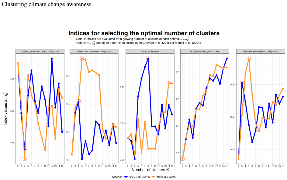
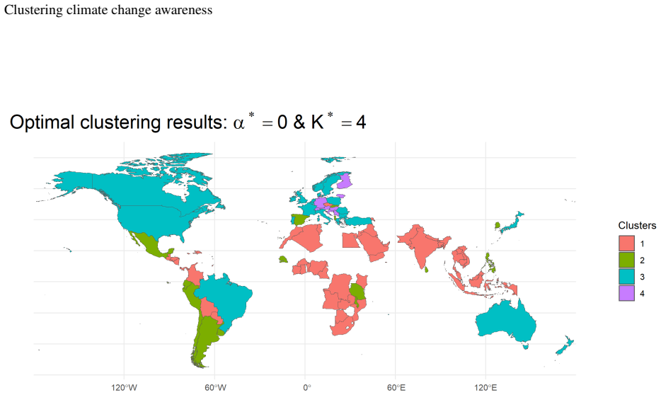
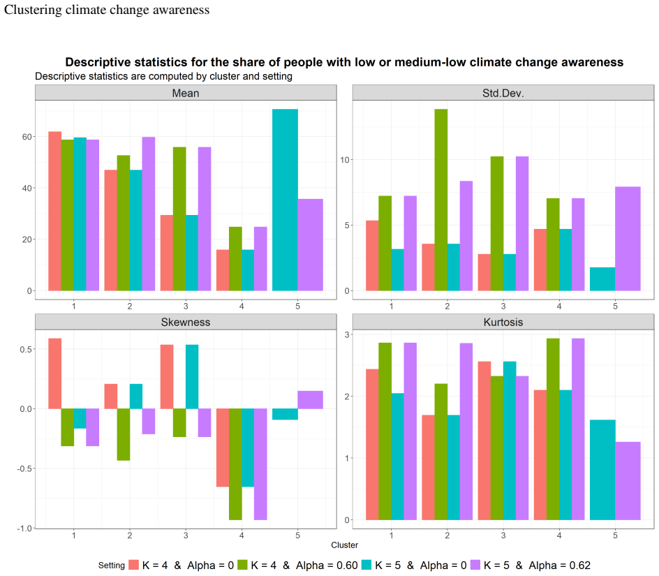
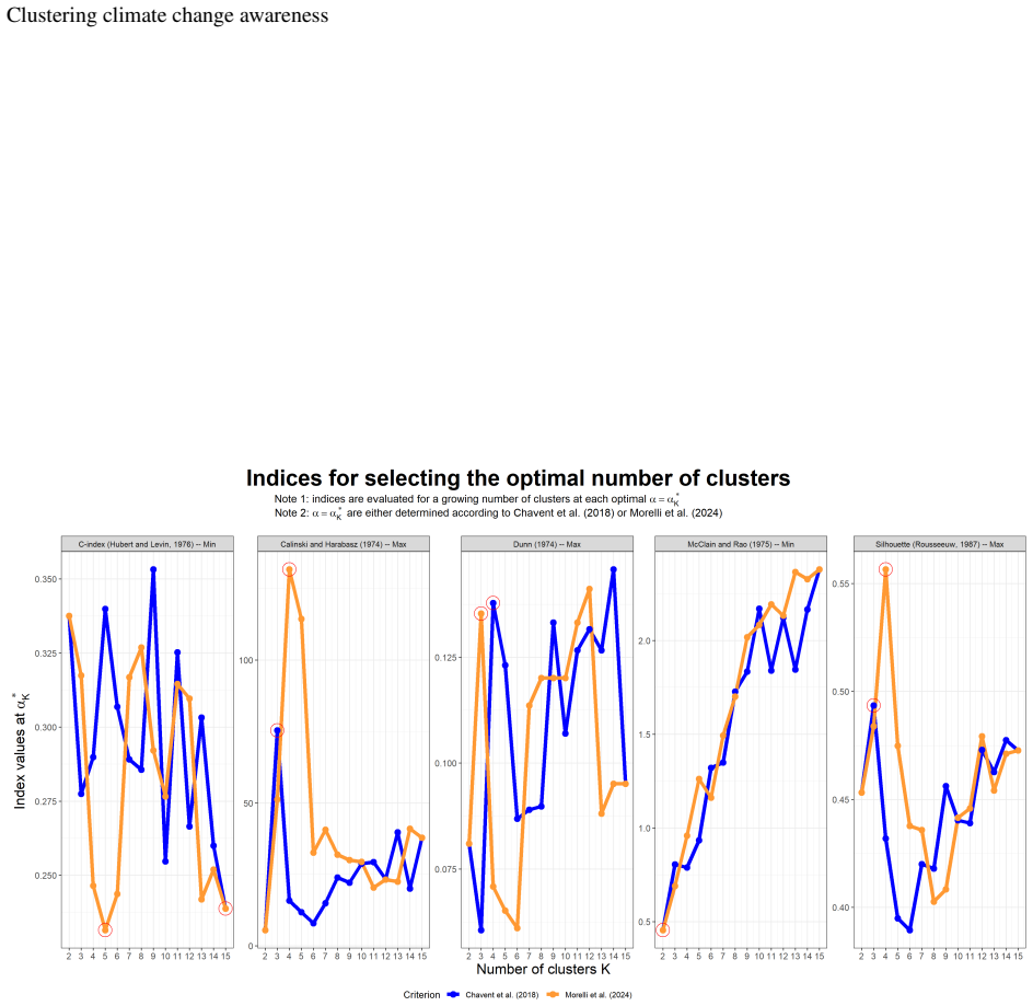
Allan David Gordon. Classification. CRC Press, 1999. 18 Clustering climate change awareness A Main analysis results: spatial hierarchical clustering using low and medium-low climate change awareness information Figure 13: Optimal values of the mixing parameter α conditioning on K clusters (that is, α∗ K) obtained using the criterion by Morelli et al. (202...
work page 1999
discussion (0)
Sign in with ORCID, Apple, or X to comment. Anyone can read and Pith papers without signing in.