REVIEW 3 major objections 5 minor 43 references
Bifurcation analysis of a prey-predator model with predator intra-specific interactions and ratio-dependent functional response
T0 review · 3 major / 5 minor · reviewed 2026-08-14 · deepseek-v4-flash
Pith's one-line read Two coexistence states appear when predators limit their own numbers
desk verdict Solid stability analysis for the two-equilibrium Bazykin model, but the Hopf/BT theorems rest on unverified algebra and the homoclinic claim overreaches. read the letter →
The pith
A machine-rendered reading of the paper's core claim, the machinery that carries it, and where it could break.
The reading
What carries the argument
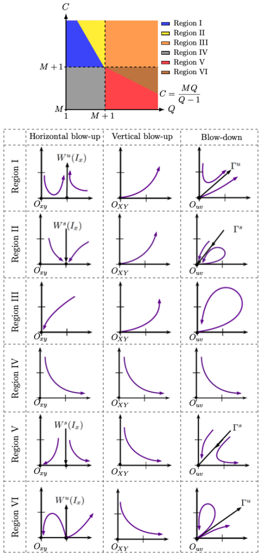
The argument runs on the Jacobian of the nondimensionalized system at interior equilibria and on three algebraic objects: the discriminant $\Delta=(M-N)^2-4N\Sigma_2$, which decides whether the two equilibria exist and when they merge; the trace function $T(u,v)$ in (20), whose sign at $P_2$ fixes stability and whose zero set is the Hopf curve; and the first Lyapunov coefficient $l_1$ in (35), whose sign tells whether the Hopf bifurcation is supercritical or subcritical. For the Bogdanov-Takens bifurcation, the load-bearing object is the map $\Psi=(X,T,D)$ from phase space and parameters to the vector field, its trace, and its determinant; the transversality condition is the nonvanishing of $G_1$ in (40), and the normal-form nondegeneracy is expressed through $G_2$, $G_3$, and $G_4$ in (42)-(44). Near the origin, the proof uses horizontal and vertical blow-ups, which transform the degenerate equilibrium into hyperbolic saddle and node points whose analysis yields the six regional phase portraits of Theorem 3.1.
What would settle it
Recompute $l_1$ and $G_1$ with a symbolic algebra system at a concrete parameter point, for example $(C,M,N)=(0.363,0.16,0.25)$ on the Hopf curve $Q\approx 1.7$, and compare the predicted stability of the bifurcating limit cycle with numerical continuation. If $l_1$'s sign differs from the paper's classification, the Hopf bifurcation would be supercritical where the paper says subcritical or vice versa; if $G_1$ vanishes, the claimed Bogdanov-Takens point would be degenerate and the codimension-two bifurcation would not occur.
Extended reading notes
Core claim
The paper's main result is a bifurcation theorem for the nondimensionalized system (3): for $Q>1$ and $C>M$, the first quadrant can contain two positive equilibria $P_1$ and $P_2$. $P_1$ is always a saddle (Theorem 3.2); $P_2$ is asymptotically stable when the trace $T(u_2,v_2)$ is negative, repelling when it is positive, and a weak focus when the trace vanishes (Theorem 3.3). The discriminant $\Delta=0$ marks the collision of $P_1$ and $P_2$ into a single equilibrium $E$, where a saddle-node bifurcation occurs provided condition (24) holds (Theorem 4.1); when, in addition, the trace of $E$ vanishes, a codimension-two Bogdanov-Takens bifurcation occurs provided the genericity conditions $G_1,G_2,G_3,G_4\neq 0$ hold (Theorem 4.3). The Hopf bifurcation at $P_2$ is codimension-one, with the sign of the first Lyapunov quantity $l_1$ in (35) determining whether the bifurcating limit cycle is stable (supercritical, $l_1<0$) or unstable (subcritical, $l_1>0$) (Theorem 4.2). The paper also claims, based on phase-plane analysis and numerical continuation, that the stable manifold of $P_1$ can close into a homoclinic curve that breaks into an unstable limit cycle (Lemma 3.3), and that the continuation of the Hopf curve reveals a Bautin point (a degenerate Hopf point where the first Lyapunov coefficient vanishes) with regions of two concentric limit cycles.
Load-bearing premise
The load-bearing premise is that the algebraic identities for the first Lyapunov coefficient $l_1$ (equation 35) and for the transversality expression $G_1$ (equation 40) are correct; the paper states these are obtained by 'straightforward substitution' and 'the derivation in [40]', but provides no derivation or computer algebra verification, so an error in either would break the Hopf or Bogdanov-Takens conclusions.
Editorial extensions
If this is right
- For parameter values below the saddle-node curve, the model always has two interior equilibria, and the stable manifold of the saddle $P_1$ separates the basins of attraction of extinction $(0,0)$ and coexistence $P_2$, making the outcome depend on initial population sizes.
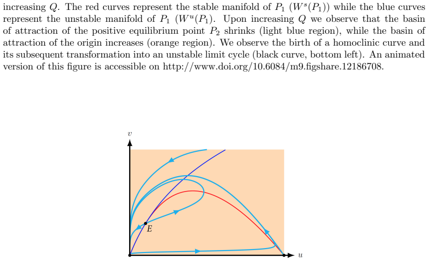
- Increasing the rescaled predation rate $Q$ moves the stable manifold of $P_1$ downward, shrinking the basin of attraction of $P_2$ until a homoclinic connection forms; further increases break the connection into an unstable limit cycle, and eventually $P_2$ loses stability through Hopf, leaving extinction as the global attractor.
- The Hopf bifurcation creates a limit cycle around $P_2$ whose stability is set by the sign of the first Lyapunov coefficient; near the Bautin point a second limit cycle is born, producing regions with two concentric cycles around the coexistence equilibrium.
- At the Bogdanov-Takens point the curves of saddle-node, Hopf, and homoclinic bifurcations meet, so the full bifurcation diagram in the $(Q,C)$-plane is organized by this codimension-two point.
- Because the smooth one-to-one change of variables used to nondimensionalize the model preserves the direction of time, all of these bifurcations carry over to the original ecological parameters, so changes in the predator per-capita consumption rate or the conversion efficiency can be read directly from the $(Q,C)$ diagram.
Reading between the lines
- The paper leaves $l_1$ and $G_1$ unverified algebraically; checking them is the cheapest way to test the Hopf and Bogdanov-Takens claims, since a sign error would flip the stability of the bifurcating limit cycles or destroy the transversality condition.
- The homoclinic bifurcation is asserted from phase-plane orientation and continuation rather than proved; an explicit calculation of the splitting distance along the would-be homoclinic orbit would turn it into a parameter curve.
- The two different two-limit-cycle configurations seen for $C=0.363$ and $C=0.6$ suggest a higher-codimension organizing center whose second Lyapunov coefficient vanishes; locating that center would unify the two phase portraits.
Signed reviews
Editorial analysis
A structured set of objections, weighed in public.
Referee Report
Summary. The manuscript studies a Bazykin prey-predator model with ratio-dependent functional response and predator intraspecific interactions. After nondimensionalizing to system (3), it classifies equilibria, proves local stability (Theorems 3.1--3.5), and derives conditions for saddle-node, Hopf, and Bogdanov-Takens bifurcations (Theorems 4.1--4.3). It also claims homoclinic bifurcations (Lemma 3.3) and uses MATCONT continuation and phase-plane simulations to illustrate basins of attraction and the impact of the predation rate and conversion efficiency.
Significance. If the algebraic identities in Sections 4.2 and 4.3 are correct, the paper is a useful contribution to the ecological-modeling literature. The stability analysis is rigorous and largely self-contained, the saddle-node proof via Sotomayor's theorem is clearly executed, and the numerical bifurcation diagrams give a valuable global picture. The main risk is not the modeling or the numerical exploration but the unverified expressions for the first Lyapunov quantity and the Bogdanov-Takens transversality condition, together with an overclaimed homoclinic-bifurcation proof.
major comments (3)
- [4.2, Eq. (35)] The first Lyapunov quantity l1 is presented as the result of "straightforward substitution" into the derivation in [40], but no derivation, computer algebra output, or verification file is supplied. Since the sign of l1 determines whether the Hopf bifurcation is supercritical or subcritical and hence whether the bifurcating limit cycle is stable or unstable, Theorem 4.2 is not fully established as written. Please provide a reproducible computer algebra derivation or an independent exact verification of (35).
- [4.3, Eq. (40)] The Bogdanov-Takens transversality condition reduces to G1 != 0, where G1 is a very large expression containing nested radicals. The text states that "straightforward substitution and algebraic simplification" gives this expression, but no derivation or code is provided. Because G1 is the only nondegeneracy check that rules out failure of the map Psi, Theorem 4.3 depends on an unverified algebraic identity. A machine-checkable derivation of (40) is needed before the Bogdanov-Takens result can be considered proven.
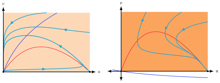
- [3.1.2, Lemma 3.3 and Abstract] The abstract states that homoclinic bifurcations are proven, but Lemma 3.3 is not proved. The text preceding it gives a continuity argument and appeals to Figures 4 and 5, and the homoclinic curve in Figure 10 comes from numerical continuation. These are numerical and heuristic evidence, not a proof. Either supply a proof of Lemma 3.3, or revise the abstract and Section 5 so that homoclinic bifurcations are described as numerically evidenced rather than proven.
minor comments (5)
- [2, Eq. (2)] The definition tau = rKt/(N + aP) in equation (2) cannot be correct, since tau would depend on the state variables; the later equations correspond to tau = rt. Please correct the nondimensionalization.
- [5, Conclusions] There is a duplicated sentence fragment: "we observe the extinction of both populationswe observe the extinction of both populations". Please fix this typographical error.
- [4.2, after Eq. (34)] The quantity G(U,V) is used in equations (33) and (34) but is defined only after those equations. Define G before first use.
- [4.3, Step 1] The statement of Theorem 4.3 lists G1,2,3,4 != 0, but the theorem statement cites (42)--(44) for G2, G3, G4; equation (42) contains an unclosed parenthesis, which should be corrected for readability.
- [3.1, Theorem 3.1] The six regions I--VI are used in the theorem before they are defined; they are defined only in the surrounding text and Figure 3. Please state the region definitions explicitly in or immediately before the theorem.
Circularity Check
No circular derivation: bifurcation conditions are explicit algebraic consequences of the model equations; unverified algebraic expressions are correctness risks, not circularity.
full rationale
The derivation chain is self-contained. The existence and number of interior equilibria are obtained by solving the nullcline equations, reducing to quadratics (6) and (8), with discriminant Δ (11); stability in Theorems 3.2–3.5 is computed directly from the Jacobian (19), determinant and trace (20). The saddle-node theorem uses Sotomayor's theorem with explicit eigenvectors and the Hessian evaluated at E; the nonzero condition (24) is stated and verified in the text. The Hopf analysis is a standard equilibrium-coordinate parameterization Ψ: (C,M,U,V)→(C,M,N,Q); system (25) is C∞-equivalent to (3) and has (U,V) as an equilibrium by construction, so the condition T(C,M,U,V)=0 (27) and DH>0 place the eigenvalues on the imaginary axis, and the Lyapunov quantity l1 in (35) is an explicit substitution into the classical Guckenheimer–Holmes formula [40], not an input to the model. The Bogdanov–Takens verification uses the standard normal-form conditions with explicit nondegeneracy expressions G1–G4 from the determinant of DΨ and Taylor coefficients. Self-citations ([28,33,37,38]) are used for boundedness/invariant-region arguments and for a heuristic homoclinic-manifold discussion; they are not used to import the saddle-node, Hopf, or BT conclusions. Two non-circular caveats: l1 (35) and G1 (40) are presented after 'straightforward substitution' with no CAS output, so algebraic-error risk exists; and Lemma 3.3's homoclinic statement is asserted from continuity/numerics rather than a complete proof, so the abstract's 'proven homoclinic bifurcations' is an overclaim. Neither constitutes equivalence between conclusion and input.
Assumptions & free parameters
assumptions (4)
- standard math Standard bifurcation theorems (Hartman-Grobman, Sotomayor's theorem, Hopf normal form, Bogdanov-Takens normal form) apply to the smooth vector field (3).
- standard math The state-dependent time rescaling phi in (2) preserves the phase portrait and orientation of (1).
- domain assumption The ecological assumptions underlying the Bazykin model (logistic prey growth, ratio-dependent functional response, intraspecific predator competition) are reasonable.
- domain assumption The analysis is restricted to the parameter regime Q > 1 and C > M, where two interior equilibria can exist.
Cite this review
Pith. "Pith review of Bifurcation analysis of a prey-predator model with predator intra-specific interactions and ratio-dependent functional response." pith.science (2026). https://pith.science/paper/YRMYOEKB
@misc{pith2026190806579,
  author       = {Pith},
  title        = {Pith review of: Bifurcation analysis of a prey-predator model with predator intra-specific interactions and ratio-dependent functional response},
  year         = {2026},
  howpublished = {\url{https://pith.science/paper/YRMYOEKB}},
  note         = {Machine review of arXiv:1908.06579}
}
read the original abstract
We study the Bazykin predator-prey model with predator intraspecific interactions and ratio-dependent functional response and show the existence and stability of two interior equilibrium points. We prove that the model displays a wide range of different bifurcations, such as saddle-node bifurcations, Hopf bifurcations, homoclinic bifurcations and Bogdanov-Takens bifurcations. We use numerical simulations to further illustrate the impact changing the predator per capita consumption rate has on the basin of attraction of the stable equilibrium points, as well as the impact of changing the efficiency with which predators convert consumed prey into new predators.
Figures

Figures from the paper (10 more)




Reference graph
Works this paper leans on
-
[40]
J. Guckenheimer and P. Holmes. Nonlinear oscillations, dynamical systems and bifurcations of vector fields. J. Appl. Mech, 51:pp. 947, 1984
work page 1984
-
[1]
A. Lotka. Contribution to the theory of periodic reactions. The Journal of Physical Chemistry, 14:271–274, 1910
work page 1910
-
[2]
P. Turchin. Complex population dynamics: a theoretical/empirical synthesis, volume 35 of Monographs in population biology. Princeton University Press, Princeton, N.J., 2003
work page 2003
-
[3]
P. Aguirre, J. Flores, and E. Gonz´ alez-Olivares. Bifurcations and global dynamics in a predator–prey model with a strong allee effect on the prey, and a ratio-dependent functional response. Nonlinear Analysis: Real World Applications, 16:235–249, 2014
work page 2014
-
[4]
R. Georgescu and A. Georgescu Some results on the dynamics generated by the Bazykin model. Atti della Accademia Peloritana dei Pericolanti-Classe di Scienze Fisiche, Matematiche e Naturali, 84:1–9, 2006
work page 2006
-
[5]
D. Greenhalgh and M Haque. A predator–prey model with disease in the prey species only. Mathematical Methods in the Applied Sciences, 30:911–929, 2007
work page 2007
-
[6]
M. Haque and E. Venturino. An ecoepidemiological model with disease in predator: the ratio- dependent case. Mathematical methods in the Applied Sciences, 30:1791–1809, 2007
work page 2007
-
[7]
Y. Xiao and L. Chen. A ratio-dependent predator–prey model with disease in the prey. Applied Mathematics and Computation, 131:397–414, 2002
work page 2002
Show all 43 references
-
[8]
Banerjee and S
M. Banerjee and S. Abbas. Existence and non-existence of spatial patterns in a ratio-dependent predator–prey model. Ecological complexity, 21:199–214, 2015
2015
-
[9]
Bartumeus, D
F. Bartumeus, D. Alonso, and J. Catalan. Self-organized spatial structures in a ratio-dependent predator–prey model. Physica A: Statistical Mechanics and its Applications, 295:53–57, 2001
2001
-
[10]
Shi and Y
H. Shi and Y. Li. Global asymptotic stability of a diffusive predator–prey model with ratio-dependent functional response. Applied Mathematics and Computation, 250:71–77, 2015
2015
-
[11]
V´ azquez-Medina, A
R. V´ azquez-Medina, A. Ledesma-Dur´ an, and J. Arag´ on. Patchy spread patterns in three-species bistable systems with facultative mutualism. Biosystems, 177:24–33, 2019
2019
-
[12]
Arditi and L
R. Arditi and L. Ginzburg. How species interact: altering the standard view on trophic ecology. Oxford University Press, 2012
2012
-
[13]
Cosner, D
C. Cosner, D. Angelis, J. Ault, and D. Olson. Effects of spatial grouping on the functional response of predators. Theoretical Population Biology, 56:65–75, 1999
1999
-
[14]
Arditi and H
R. Arditi and H. Saiah. Empirical evidence of the role of heterogeneity in ratio-dependent consump- tion. Ecology, 73:1544–1551, 1992
1992
-
[15]
Gutierrez
A. Gutierrez. Physiological basis of ratio-dependent predator-prey theory: the metabolic pool model as a paradigm. Ecology, 73:1552–1563, 1992
1992
-
[16]
Kuang and E
Y. Kuang and E. Beretta. Global qualitative analysis of a ratio-dependent predator–prey system. Journal of mathematical biology, 36:389–406, 1998
1998
-
[17]
Jost and R
C. Jost and R. Arditi. Identifying predator–prey processes from time-series. Theoretical population biology, 57:325–337, 2000
2000
-
[18]
Rosenzweig
M. Rosenzweig. Paradox of enrichment: destabilization of exploitation ecosystems in ecological time. Science, 171:385–387, 1971
1971
-
[19]
Berryman
A. Berryman. The orgins and evolution of predator-prey theory. Ecology, 73:1530–1535, 1992
1992
-
[20]
R. Luck. Evaluation of natural enemies for biological control: a behavioral approach. Trends in Ecology & Evolution, 5:196–199, 1990
1990
-
[21]
Bazykin, A
A. Bazykin, A. Khibnik, and B. Krauskopf. Nonlinear dynamics of interacting populations, volume 11. World Scientific, Singapore, 1998
1998
-
[22]
Aguirre, E
P. Aguirre, E. Gonz´ alez-Olivares, and E. S´ aez. Two limit cycles in a Leslie–Gower predator–prey model with additive Allee effect. Nonlinear Analysis: Real World Applications, 10:1401–1416, 2009
2009
-
[23]
Flores and E
J. Flores and E. Gonz´ alez-Olivares. Dynamics of a predator–prey model with allee effect on prey and ratio–dependent functional response. Ecological Complexity, 18:59–66, 2014
2014
-
[24]
R. Liu, D. DeAngelis, and J Bryant. Ratio-dependent functional response emerges from optimal foraging on a complex landscape. Ecological modelling, 292:45–50, 2014
2014
-
[25]
Abrams and L
P. Abrams and L. Ginzburg. The nature of predation: prey dependent, ratio dependent or neither? Trends in Ecology & Evolution, 15:337–341, 2000
2000
-
[26]
M. Haque. Ratio-dependent predator-prey models of interacting populations. Bulletin of mathematical biology, 71:430–452, 2009
2009
-
[27]
Arancibia-Ibarra
C. Arancibia-Ibarra. The basins of attraction in a Modified May-Holling-Tanner predator-prey model with Allee effect. Nonlinear Analysis: Theory, Methods & Applications, 185:15–28, 2019
2019
-
[28]
Arancibia-Ibarra, J
C. Arancibia-Ibarra, J. Flores, M. Bode, G. Pettet, and P. van Heijster. A modified may–holling– tanner predator-prey model with multiple allee effects on the prey and an alternative food source for the predator. Discrete & Continuous Dynamical Systems-B, 22:1–20, 2020
2020
-
[29]
Gonz´ alez-Olivares, C
E. Gonz´ alez-Olivares, C. Arancibia-Ibarra, A. Rojas-Palma, and B. Gonz´ alez-Ya˜ nez. Bifurcations and multistability on the May–Holling–Tanner predation model considering alternative food for the predators. Mathematical Biosciences and Engineering, 16:4274–4298, 2019
2019
-
[30]
Andronov
A. Andronov. Qualitative theory of second-order dynamic systems, volume 22054. Halsted Press, 1973
1973
-
[31]
C. Chicone. Ordinary Differential Equations with Applications, volume 34 of Texts in Applied Mathematics. World Scientific, Springer-Verlag New York, 2006
2006
-
[32]
Dumortier, J
F. Dumortier, J. Llibre, and J. Art´ es. Qualitative theory of planar differential systems. Springer Berlin Heidelberg, Springer-Verlag Berlin Heidelberg, 2006
2006
-
[33]
Arancibia-Ibarra, J
C. Arancibia-Ibarra, J. Flores, G. Pettet, and P. van Heijster. A Holling–Tanner predator–prey model with strong Allee effect. International Journal of Bifurcation and Chaos, 29(11):1–16, 2019
2019
-
[34]
Freedman
H. Freedman. Deterministic mathematical models in population ecology. Pure and applied mathe- matics (Dekker); 57. Wiley, New York, 1980
1980
-
[35]
Berezovskaya, G
F. Berezovskaya, G. Karev, and R. Arditi. Parametric analysis of the ratio-dependent predator–prey model. Journal of Mathematical Biology, 43:221–246, 2001
2001
-
[36]
Berezovskaya, A
F. Berezovskaya, A. Novozhilov, and G. Karev. Population models with singular equilibrium. Mathematical biosciences, 208:270–299, 2007
2007
-
[37]
Flores and E
J. Flores and E. Gonz´ alez–Olivares. A modified Leslie—Gower predator—prey model with ratio- dependent functional response and alternative food for the predator. Mathematical Methods in the Applied Sciences, 40:2313–2328, 2017
2017
-
[38]
Aguirre, E
P. Aguirre, E. Gonz´ alez-Olivares, and E. S´ aez. Three limit cycles in a Leslie–Gower predator–prey model with additive Allee effect. SIAM Journal on Applied Mathematics, 69:1244–1262, 2009
2009
-
[39]
L. Perko. Differential Equations and Dynamical Systems. Springer New York, 2001
2001
-
[41]
Kuznetsov
Y. Kuznetsov. Elements of applied bifurcation theory, volume 112. Springer Science & Business Media, 2013
2013
-
[42]
Doedel, T
E. Doedel, T. Fairgrieve, B. Sandstede, A. Champneys, Y. Kuznetsov, and X. Wang. Auto-07p: Continuation and bifurcation software for ordinary differential equations. 2007
2007
-
[43]
Dhooge, W
A. Dhooge, W. Govaerts, and Y. Kuznetsov. Matcont: a matlab package for numerical bifurcation analysis of odes. ACM Transactions on Mathematical Software (TOMS), 29:141–164, 2003
2003
Reviewed August 14, 2026 · model on record in the stance chip above.
Discussion (0). Continue with ORCID to comment.