REVIEW 5 major objections 9 minor 31 references
A Semiparametric Stochastic Volatility Model with Dependent Errors
T0 review · 5 major / 9 minor · reviewed 2026-08-07 · deepseek-v4-flash
Pith's one-line read Semiparametric SV model with dependent errors lowers estimation bias
desk verdict A genuine but incremental extension of the authors' NSVM work, undermined by a self-contradictory volatility comparison and an incoherent plug-in posterior. read the letter →
The pith
A machine-rendered reading of the paper's core claim, the machinery that carries it, and where it could break.
The reading
What carries the argument
The load-bearing object is the bivariate kernel density estimate \(\hat{k}\) of the joint error density of \((u_t, \nu_t)\), computed with the kde2d routine on standardized residuals from an initial Gaussian SV fit. This estimate is plugged directly into the volatility posterior in place of the two Gaussian factors, giving \(p(h_t \mid \ldots) \propto $h_t^{{-3/2}}$ \hat{k}(y_t / \sqrt{h_t}, (\ln h_t - \mu_t)/\sigma_\nu)\). The inverse-gamma proposal distribution is retained to drive an efficient Metropolis-Hastings sampler for the latent volatilities.
What would settle it
Generate data from a bivariate normal error process with independent errors and compare the empirical coverage of NSVM-3's posterior credible intervals for the parameters and volatility against the nominal level; if the plug-in kernel step destroys posterior coherence, the coverage will drift systematically while the Gaussian model's intervals remain calibrated.
Extended reading notes
Core claim
The paper's central discovery is that replacing the Gaussian densities for the return error and the volatility error in the volatility posterior with a bivariate kernel density estimate of their joint distribution—estimated from residuals of a preliminary Gaussian SV fit—produces more accurate parameter and volatility estimates. In simulations with correlated Gaussian errors and with bivariate Student-t errors, NSVM-3 attains the lowest square root mean squared error for the persistence parameter, the level parameter, and the volatility-of-volatility parameter, and it generally produces lower volatility estimation error than the Gaussian SV model and a popular Bayesian implementation. The empirical application to S&P 500 daily returns shows volatility estimates that react more markedly to large price movements, suggesting the model captures real market behavior that Gaussian assumptions miss.
Load-bearing premise
The posterior treats the kernel density estimate, built from residuals of a preliminary Gaussian fit on the same data, as the exact joint density of the error terms; nothing adjusts for the uncertainty in that estimate, so the MCMC samples may not come from a coherent posterior of a well-defined semiparametric model.
Editorial extensions
If this is right
- Practitioners can estimate stochastic volatility models without committing to a parametric family for the error distributions while still allowing dependence between return and volatility shocks.
- The method extends the semiparametric approach to settings where the error dependence structure is unknown and must be learned from data.
- The simulation results quantify concrete gains in parameter bias and variance for persistence, level, and volatility-of-volatility under both Gaussian and heavy-tailed dependent errors.
- The S&P 500 application demonstrates that the semiparametric volatility estimates respond more strongly to large market moves, which could inform risk management and option pricing.
- The framework opens the door to fully data-driven error distributions in other state-space and latent-variable models beyond stochastic volatility.
Reading between the lines
- If the plug-in kernel step is not corrected, the reported gains may partly reflect MCMC sampling from a pseudo-posterior rather than a coherent Bayesian model; a two-stage or Dirichlet-process mixture prior would be a direct testable fix.
- A natural stress test would compare out-of-sample predictive log-likelihoods on held-out periods, since in-sample parameter error does not directly measure forecasting performance.
- The approach could be extended to multivariate or multi-asset volatility models, where a joint nonparametric error density would capture cross-asset tail dependence in a purely data-driven way.
Editorial analysis
A structured set of objections, weighed in public.
Referee Report
Summary. The paper proposes NSVM-3, a semiparametric stochastic volatility model in which the joint density of the return innovation and the volatility innovation is estimated nonparametrically by a bivariate kernel density estimate, thereby allowing for non-Gaussianity and dependence between the two error processes. The method is implemented by replacing the Gaussian components in the full conditional posterior for the latent volatility with the kernel density estimate, while the model parameters are sampled from conditional posteriors derived under the Gaussian model. The paper compares NSVM-3 against a Gaussian SV model and the R package stochvol in simulations with dependent Gaussian and Student-t errors, reporting lower square-root mean squared errors for parameters and, allegedly, for volatility estimates. An empirical application to S&P 500 daily returns is presented as an illustration. The central methodological and empirical claims are, however, not supported by the evidence in the manuscript.
Significance. The topic is relevant: relaxing both the distributional and the independence assumptions on the shocks of a stochastic volatility model is a natural extension, and a well-posed semiparametric Bayesian procedure could be of value to financial econometrics. The paper also has a constructive element: it provides a full MCMC algorithm and presents simulation and empirical comparisons. But the manuscript as it stands does not establish a coherent inferential target: the plug-in kernel density in Eq. (12) is treated as the true error density without correction for estimation from the same data, the parameter samplers do not use the semiparametric likelihood, and the reported volatility-accuracy claim is directly contradicted by the paper's own tables. With a properly derived posterior and a fairer comparison design the idea might become publishable, but the current version does not provide a valid basis for the claimed advantages.
major comments (5)
- [Section 3, Eq. (12)] The posterior target in Eq. (12) uses a bivariate kernel density estimate \hat{k} that is constructed from standardized residuals \hat{u}_t and \hat{w}_t obtained from a preliminary Gaussian SV fit on the same dataset. This estimate is plugged into the full conditional of h_t as if it were the exact joint density of (u_t, \nu_t). No correction is made for the fact that \hat{k} is estimated from the data, and no consistency, coverage, or Bernstein-von Mises type result is provided. Consequently, the MCMC samples produced by Algorithms 2 and 4 are not draws from a well-defined posterior distribution of the semiparametric model; they are draws from a procedure that uses the data twice. This is a load-bearing issue because the entire inference, including the parameter and volatility estimates in Tables 1-4, depends on this target.
- [Section 4.1, Algorithms 3, 7, and 8] The samplers for \delta, \alpha, and \sigma_\nu use the conditional posterior distributions derived from the Gaussian parametric model in Eqs. (5)-(7), and Algorithm 3 explicitly states that 'Let p be the posterior distribution in a parametric setting.' Thus the parameter estimates reported in Tables 1 and 2 are not estimates under the semiparametric model with dependent, nonparametrically distributed errors; they are Gaussian-model estimates. The paper therefore provides no evidence that the proposed semiparametric framework improves parameter estimation, because the parameters are not actually being estimated from the semiparametric likelihood.
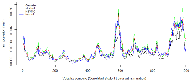
- [Section 5.3, Tables 3 and 4] The text claims that 'Tables 3, 4 indicate that NSVM-3 generally produces lower ... mean absolute percentage error (MAPE),' but this is contradicted by the numbers in the tables. In Table 3, NSVM-3 has the largest MAPE for all three posterior summaries (0.09959, 0.09939, 0.09944) compared to stochvol (0.09945, 0.09927, 0.09912) and Gaussian (0.09932, 0.09908, 0.09922). In Table 4, NSVM-3's MAPE values (0.09949, 0.09959, 0.09966) are slightly worse than stochvol's (0.09948, 0.09957, 0.09965). The srMSE and MAE differences are in the fifth decimal place (e.g., 0.008250 vs 0.008252) and are reported without standard errors or significance tests across the 100 runs. The claim of superior volatility estimation, which is central to the paper's conclusion, is therefore not supported by the presented results.
- [Sections 5.1 and 5.2] The simulation comparison omits a parametric baseline that allows for correlation between the error terms. The data are generated with \rho(u_t, \nu_t) = -0.5, yet the two comparators (the Gaussian SV model and the stochvol implementation as used here) assume independent errors. A natural baseline would be a parametric SV model with bivariate Gaussian or bivariate Student-t errors and an estimated correlation parameter. Without such a baseline, the reported gains of NSVM-3 in parameter srMSE and in volatility error metrics could be attributed entirely to the inclusion of dependence rather than to the nonparametric flexibility of the error density. The paper never reports an estimate of the correlation parameter, so this alternative explanation is not addressed.
- [Section 6] The empirical application to the S&P 500 does not provide any quantitative measure of volatility estimation accuracy. Since the true volatility is unobserved in real data, the visual comparison in Figure 10 cannot establish that NSVM-3 'responds more accurately' to large fluctuations. No model comparison metrics, such as predictive likelihoods, coverage, or out-of-sample losses, are reported. The empirical claim is therefore not substantiated beyond anecdotal visual inspection.
minor comments (9)
- [Section 5.1] The text states that the simulation was repeated 50 times, and the box plots refer to that number, but the srMSE formulas and the table captions use 100 runs. Please clarify whether the results are based on 50 or 100 replications.
- [Equation (8)] The formula for s appears to contain typographical errors: the term 's1δs1' in the manuscript is not a valid expression, and the summation expressions following it are garbled. The definitions of s1, s2, s3 in Eq. (9) are clear, but Eq. (8) needs to be rewritten consistently.
- [Equation (12)] The symbol N is used both for the sample size and for the kernel function within the same equation (the kernel is written as N(x, y)), which is confusing. Use a different letter, e.g., K, for the kernel.
- [Section 4.1] The tuning constant c* is stated to be 1.2 in the text, but Algorithm 5 and the later algorithms use log(1.1) in the code-like pseudocode. The relationship between c* and the 1.1 factor should be explained or made consistent.
- [Section 4.1, Eq. (14)] The definition of c uses h_m as the mode of q, but in Algorithm 2 the acceptance steps use a constant c that is defined after its first use in the pseudocode. Reordering the algorithm so that c is computed before the proposal step would improve readability.
- [Abstract and Sections 5.1-5.2] The abstract claims lower 'bias and variance,' but the paper only reports srMSE, which combines bias and variance. Reporting bias and variance separately, or at least stating that srMSE is a combined measure, would be more precise.
- [Section 4] No convergence diagnostics are reported for the MCMC chains, such as trace plots, effective sample sizes, or Gelman-Rubin statistics. Given the nontrivial proposal mechanism, the reader cannot assess whether the MCMC results in Tables 1-4 are reliable.
- [Section 4, Algorithm 1] Algorithm 1 is only a sketch and references parameters 'T' and 'b' that are not defined in the main text (likely burn-in and total iterations). These should be defined explicitly in the algorithm caption.
- [References] The reference to 'Feng and Gangopadhyay (2025)' is cited as an arXiv preprint without a full citation or version; the reader cannot easily locate or verify the claimed methodological relationship.
Circularity Check
No significant circularity; the plug-in kernel likelihood is not a definitional identity with the reported estimates.
full rationale
The paper's derivation is self-contained. The semiparametric volatility posterior in Eq. (12) is explicitly built from a bivariate kernel density estimate \hat{k} computed from residuals of a Gaussian SV fit on the same data. That is a plug-in semiparametric likelihood, not a definitional identity: \hat{k} is an estimated input, not the parameter or volatility quantity being reported, and the MCMC output is a genuinely different function of the data. Parameter conditionals (5)-(7) are standard Gaussian SV full conditionals; using them for \delta, \alpha and \sigma_\nu while sampling h_t from the kernel-based target is an algorithmic approximation, but it does not make the reported estimates equal to the model inputs by construction. Comparisons against stochvol provide an external benchmark. The self-citations to Feng and Gangopadhyay (2025) describe prior methodology, but the present paper specifies the estimator, residuals, and algorithms itself, so those citations are not load-bearing for the derivation. The apparent MAPE inconsistency in Section 5.3 is a numerical-claim support issue, not a circularity. No load-bearing step reduces to its own inputs.
Assumptions & free parameters
free parameters (2)
- Kernel bandwidths b_x, b_y =
chosen by standard bandwidth selection via kde2d in R
- MH tuning constant c* =
1.2 in simulation text, 1.1 in appendix algorithms
assumptions (4)
- ad hoc to paper The bivariate kernel density estimate of residuals is a valid approximation of the true joint error density and can be plugged into the posterior target without correction.
- ad hoc to paper Conditional posterior distributions for δ, α, and σν derived from the Gaussian model remain valid in the semiparametric model.
- domain assumption The AR(1) log-volatility process with |δ| < 1 is stationary and identifiable.
- standard math Kernel density estimation is reliable at N=500 with the chosen bandwidth selector.
Cite this review
Pith. "Pith review of A Semiparametric Stochastic Volatility Model with Dependent Errors." pith.science (2026). https://pith.science/paper/YX4YPSB6
@misc{pith2026250601094,
  author       = {Pith},
  title        = {Pith review of: A Semiparametric Stochastic Volatility Model with Dependent Errors},
  year         = {2026},
  howpublished = {\url{https://pith.science/paper/YX4YPSB6}},
  note         = {Machine review of arXiv:2506.01094}
}
read the original abstract
This paper proposes a semiparametric stochastic volatility (SV) model that relaxes the restrictive Gaussian assumption in both the return and volatility error terms, allowing them to follow flexible, nonparametric distributions with potential dependence. By integrating this framework into a Bayesian Markov Chain Monte Carlo (MCMC) approach, the model effectively captures the heavy tails, skewness, and other complex features often observed in financial return data. Simulation studies under correlated Gaussian and Student's t error settings demonstrate that the proposed method achieves lower bias and variance when estimating model parameters and volatility compared to traditional Gaussian-based and popular Bayesian implementations. We conduct an empirical application to the real world financial data, which further underscores the model's practical advantages: it provides volatility estimates that respond more accurately to large fluctuations, reflecting real-world market behavior. These findings suggest that the introduced semiparametric SV framework offers a more robust and adaptable tool for financial econometrics, particularly in scenarios characterized by non-Gaussian and dependent return dynamics.
Figures


Figures from the paper (8 more)




Reference graph
Works this paper leans on
-
[1]
Abanto-Valle, C., Migon, H., and Lachos, V. (2011). Stochastic volatility in mean models with scale mixtures of normal distributions and correlated errors: A bayesian approach. Journal of Statistical Planning and Inference , 141(5):1875--1887
work page 2011
-
[2]
Barndorff-Nielsen, O. E. (1997). Normal inverse gaussian distributions and stochastic volatility modelling. Scandinavian Journal of Statistics , 24(1):1--13
1997
-
[3]
and Scholes, M
Black, F. and Scholes, M. (1973). The pricing of options and corporate liabilities. Journal of Political Economy , 81(3):637--654
1973
-
[4]
Carter, C. K. and Kohn, R. (1994). On gibbs sampling for state space models. Biometrika , 81(3):541--553
1994
-
[5]
Chesney, M. and Scott, L. (1989). Pricing european currency options: A comparison of the modified black- scholes model and a random variance model. The Journal of Financial and Quantitative Analysis , 24(3):267--284
work page 1989
-
[6]
David Chan, R. K. and Kirby, C. (2006). Multivariate stochastic volatility models with correlated errors. Econometric Reviews , 25(2-3):245--274
work page 2006
-
[7]
Di, J. and Gangopadhyay, A. (2011). On the efficiency of a semi‐parametric garch model. The Econometrics Journal , 14(2):257--277
work page 2011
-
[8]
Di, J. and Gangopadhyay, A. (2013). One-step semiparametric estimation of the garch model. Journal of Financial Econometrics , 12(2):382--407
work page 2013
Show all 31 references
-
[9]
and Gangopadhyay, A
Di, J. and Gangopadhyay, A. (2015). A data-dependent approach to modeling volatility in financial time series. Sankhyā: The Indian Journal of Statistics, Series B (2008-) , 77(1):1--26
2015
-
[10]
Doan, T., Jacquier, E., Polson, N., and Rossi, P. (1994). Bayesian analysis of stochastic volatility models. Journal of Business & Economic Statistics , 12:371--89
1994
-
[11]
Durham, G. (2006). Monte carlo methods for estimating, smoothing, and filtering one- and two-factor stochastic volatility models. Journal of Econometrics , 133:273--305
2006
-
[12]
Eric Jacquier, N. G. P. and Rossi, P. E. (2002). Bayesian analysis of stochastic volatility models. Journal of Business & Economic Statistics , 20(1):69--87
2002
-
[13]
and Gangopadhyay, A
Feng, Y. and Gangopadhyay, A. (2025). On a semiparametric stochastic volatility model. arXiv
2025
-
[14]
C., and Renault, E
Ghysels, E., Harvey, A. C., and Renault, E. (1996). 5 Stochastic volatility , volume 14 of Handbook of Statistics , pages 119--191. Elsevier
1996
-
[15]
Harvey, A. C. and Shephard, N. (1996). Estimation of an asymmetric stochastic volatility model for asset returns. Journal of Business & Economic Statistics , 14(4):429--434
1996
-
[16]
Hastings, W. K. (1970). Monte carlo sampling methods using markov chains and their applications. Biometrika , 57(1):97--109
1970
-
[17]
and White, A
Hull, J. and White, A. (1987). The pricing of options on assets with stochastic volatilities. The Journal of Finance , 42(2):281--300
1987
-
[18]
Jacquier, E., Polson, N., and Rossi, P. (2004). Bayesian analysis of stochastic volatility models with fat-tails and correlated errors. Journal of Econometrics , 122:185--212
2004
-
[19]
Kastner, G. (2016). Dealing with stochastic volatility in time series using the r package stochvol. Journal of Statistical Software , 69(5):1–30
2016
-
[20]
Kim, S., Shephard, N., and Chib, S. (1998). Stochastic volatility: Likelihood inference and comparison with arch models. The Review of Economic Studies , 65(3):361--393
1998
-
[21]
Mahieu, R. J. and Schotman, P. C. (1998). An empirical application of stochastic volatility models. Journal of Applied Econometrics , 13(4):333--359
1998
-
[22]
Mandelbrot, B. (1963). The variation of certain speculative prices. The Journal of Business , 36:371–418
1963
-
[23]
Markowitz, H. (1952). Portfolio selection. The Journal of Finance , 7(1):77--91
1952
-
[24]
W., Rosenbluth, M
Metropolis, N., Rosenbluth, A. W., Rosenbluth, M. N., Teller, A. H., and Teller, E. (1953). Equation of state calculations by fast computing machines. The Journal of Chemical Physics , 21(6):1087--1092
1953
-
[25]
and Ranjan, P
Mukhoti, S. and Ranjan, P. (2019). A new class of discrete-time stochastic volatility model with correlated errors. Applied Economics , 51(3):259--277
2019
-
[26]
Omori, Y., Chib, S., Shephard, N., and Nakajima, J. (2007). Stochastic volatility with leverage: Fast and efficient likelihood inference. Journal of Econometrics , 140(2):425--449
2007
-
[27]
Shephard, N. (1996). Statistical aspects of ARCH and stochastic volatility , pages 1--67. Chapman & Hall
1996
-
[28]
Taylor, S. J. (1994). Modeling stochastic volatility: A review and comparative study. Mathematical Finance , 4(2):183--204
1994
-
[29]
Tierney, L. (1994). Markov Chains for Exploring Posterior Distributions . The Annals of Statistics , 22(4):1701--1728
1994
-
[30]
Tierney, L. (1998). A note on metropolis-hastings kernels for general state spaces. The Annals of Applied Probability , 8(1):1--9
1998
-
[31]
Venables, W. N. and Ripley, B. D. (2002). Modern Applied Statistics with S . Springer
2002
Reviewed August 7, 2026 · model on record in the stance chip above.
Discussion (0). Sign in to comment.