Multi-cluster chimeras in phase oscillators with repulsive nonlocal coupling
Pith reviewed 2026-05-19 18:21 UTC · model grok-4.3
pith:YYHODSXI Add to your LaTeX paper
What is a Pith Number?\usepackage{pith}
\pithnumber{YYHODSXI}
Prints a linked pith:YYHODSXI badge after your title and writes the identifier into PDF metadata. Compiles on arXiv with no extra files. Learn more
The pith
Phase oscillators with repulsive nonlocal coupling form multi-cluster chimeras where synchronized clusters differ by 2π/n.
A machine-rendered reading of the paper's core claim, the machinery that carries it, and where it could break.
Core claim
For phase oscillators on a ring with nonlocal piecewise-linear repulsive coupling that includes a fixed phase lag, the multi-cluster chimera states are characterized by n synchronized clusters whose consecutive members differ in phase by 2π/n. This antiphase or splay relation follows directly from the repulsive sign and the nonlocal spatial structure; it is confirmed both numerically and by solving the reduced equations for the cluster phases and amplitudes. Stability analysis then maps the regions of coupling strength and phase lag in which the states persist, and the Ott-Antonsen ansatz reproduces the same phase relation and stability boundaries.
What carries the argument
Multi-cluster chimera state in which n consecutive synchronized clusters maintain a fixed phase offset of 2π/n under repulsive nonlocal coupling.
If this is right
- Stability boundaries in the space of coupling strength and phase lag identify where the 2π/n states can be observed.
- The phase-offset rule is tied to the repulsive sign of the coupling and does not appear in the corresponding attractive case.
- Ott-Antonsen reduction reproduces both the phase relation and the stability regions found in direct simulation.
- The chimera states consist of n synchronized clusters coexisting with a desynchronized background.
Where Pith is reading between the lines
- The same phase-locking pattern may appear in other oscillator networks once repulsion is made spatially nonlocal.
- Changing the range or functional shape of the repulsion could produce different cluster numbers or phase offsets.
- The mechanism supplies a route to engineer partial synchronization by tuning only the sign and range of the coupling.
Load-bearing premise
The coupling function is assumed to be piecewise linear, nonlocal, repulsive, and to include a fixed phase lag.
What would settle it
A numerical integration or experiment in which the phase differences between consecutive synchronized clusters deviate from 2π/n while the coupling remains piecewise linear, nonlocal, and repulsive would falsify the central phase-relation claim.
Figures


read the original abstract
Local repulsive coupling tend to a desynchronize ensembles of globally coupled oscillators, but when the repulsive coupling is nonlocal, multi-cluster chimeras can result. In this case, several groups of synchronized oscillators (the so-called clusters) are formed, and these coexist with a set of desynchronized oscillators. For phase oscillators on a ring with nonlocal piecewise linear repulsive coupling that also involves a phase lag, we find that in the multi-cluster chimera state the synchronized clusters are either antiphase or in splay with respect to each other, namely the n consecutive synchronized clusters differ in phase by 2{\pi}/n. This is in contrast to multi-cluster chimeras that are formed with nonlocal attractive coupling. The synchronized solutions are studied numerically as well as analytically and by analysing their stability, we identify the parameter regions where these can be observed. Our numerical results are validated by dimensional reduction using the Ott-Antonsen analysis.
Editorial analysis
A structured set of objections, weighed in public.
Referee Report
Summary. The manuscript studies multi-cluster chimera states in a ring of phase oscillators with nonlocal piecewise-linear repulsive coupling that includes a fixed phase lag. Through numerical simulations, linear stability analysis of the synchronized cluster states, and Ott-Antonsen reduction, the authors report that the n synchronized clusters differ in phase by exactly 2π/n (antiphase for n=2, splay for larger n). This phase rule is contrasted with the behavior under attractive nonlocal coupling, and stable parameter regions in coupling strength and phase lag are identified.
Significance. If the central observations hold, the work supplies a concrete phase-organization rule for multi-cluster chimeras under repulsive nonlocal interactions, a regime less studied than its attractive counterpart. The combination of direct simulation, stability analysis, and dimensional reduction provides useful cross-validation, and the explicit mapping of stable regions is a practical contribution for future modeling or experiments.
major comments (1)
- [§3] §3 (model and effective interaction): the phase-difference rule and the stability of the 2π/n configurations are obtained by integrating the specific piecewise-linear kernel over the supports of the clusters. Because the sign and magnitude of these integrals are kernel-dependent, the manuscript should state explicitly that the reported rule and stability boundaries are tied to this functional form and nonlocality range; without such a statement the central claim risks being read as more general than the derivation supports.
minor comments (2)
- [Figures] Figure 4 and 5 captions: parameter values (coupling strength, phase lag, nonlocality range) used for each panel should be listed explicitly rather than referred to the text.
- [Model section] Notation: the phase lag is introduced as a fixed parameter but its symbol is not consistently defined in the first appearance in the model equation.
Simulated Author's Rebuttal
We thank the referee for the careful reading of our manuscript and the constructive comment. We agree that the results are specific to the chosen coupling kernel and have revised the text accordingly to make this explicit.
read point-by-point responses
-
Referee: [§3] §3 (model and effective interaction): the phase-difference rule and the stability of the 2π/n configurations are obtained by integrating the specific piecewise-linear kernel over the supports of the clusters. Because the sign and magnitude of these integrals are kernel-dependent, the manuscript should state explicitly that the reported rule and stability boundaries are tied to this functional form and nonlocality range; without such a statement the central claim risks being read as more general than the derivation supports.
Authors: We agree with the referee. The phase-difference rule (clusters differing by exactly 2π/n) and the associated stability boundaries are obtained by explicit integration of the piecewise-linear kernel over the cluster supports, so both the sign and magnitude of the resulting effective coupling are kernel-dependent. In the revised manuscript we have added a clarifying paragraph in §3 (and a brief remark in the abstract and conclusions) stating that the reported 2π/n organization and the identified stable regions are tied to the present functional form and nonlocality range. We also note that other kernels would in general produce different integrals and therefore different phase rules, which would need to be analyzed separately. revision: yes
Circularity Check
No circularity: phase-difference rule obtained from independent numerical and reduced analysis of given model
full rationale
The paper obtains the 2π/n inter-cluster phase offset by direct numerical integration of the phase-oscillator equations on the ring, followed by explicit linear stability analysis of the resulting cluster states and cross-validation via the standard Ott-Antonsen reduction. These operations solve the dynamical system for the chosen piecewise-linear repulsive kernel plus fixed lag; the offset is an emergent property of the solved trajectories, not a re-statement of the kernel integral or a fitted parameter renamed as a prediction. No self-citation is invoked to justify uniqueness or to close the derivation, and the Ott-Antonsen step is an external, parameter-free technique whose assumptions do not presuppose the reported phase rule. The derivation chain is therefore self-contained against the model equations themselves.
Axiom & Free-Parameter Ledger
free parameters (1)
- coupling strength and phase lag
axioms (1)
- domain assumption Ott-Antonsen reduction applies to the nonlocal repulsive kernel
Lean theorems connected to this paper
-
IndisputableMonolith/Cost/FunctionalEquation.leanwashburn_uniqueness_aczel unclear?
unclearRelation between the paper passage and the cited Recognition theorem.
the n consecutive synchronized clusters differ in phase by 2π/n ... validated by dimensional reduction using the Ott-Antonsen analysis
-
IndisputableMonolith/Foundation/AbsoluteFloorClosure.leanreality_from_one_distinction unclear?
unclearRelation between the paper passage and the cited Recognition theorem.
nonlocal piecewise linear repulsive coupling that also involves a phase lag
What do these tags mean?
- matches
- The paper's claim is directly supported by a theorem in the formal canon.
- supports
- The theorem supports part of the paper's argument, but the paper may add assumptions or extra steps.
- extends
- The paper goes beyond the formal theorem; the theorem is a base layer rather than the whole result.
- uses
- The paper appears to rely on the theorem as machinery.
- contradicts
- The paper's claim conflicts with a theorem or certificate in the canon.
- unclear
- Pith found a possible connection, but the passage is too broad, indirect, or ambiguous to say the theorem truly supports the claim.
Reference graph
Works this paper leans on
-
[1]
in terms of the components of the order parameter becomes ∂Φ( x, t ) ∂t = ω − ζ − R sin(Φ( x, t ) − Θ + α ), (3) where the phases of the oscillators are decoupled, but the oscillators still interact through the coherence parameter R and average phase Θ. G(x) -a a a a x FIG. 1: Schematic diagram showing the nonlocal piecewise linear coupling depicting loca...
-
[2]
An analogy to this kind of coupling can be found in the con- nections between cortical neurons and their neighbours, where the coupling kernel resembles “inverted Mexican- hat” like function, comprising short-range inhibition and long-range excitation or neutral connections [ 32]. The effects of repulsive nonlocal coupling on the emer- gent dynamical state...
-
[3]
The interplay of the coupling function and the phase lag parameter α gives rise to various states
and then analysing the asymptotic states. The interplay of the coupling function and the phase lag parameter α gives rise to various states. Low values of α favour synchronized states whereas α close to π/ 2 gives rise to chimeras. We fix α = 1 . 52 and study the effect of changing the form of G(x) on the emergent states. We extensively investigate different...
-
[4]
2(i)-(xxii)), for instance, Fig
When ns is small, say 2 or 3, one can clearly distinguish between local and lateral cou- plings (Fig. 2(i)-(xxii)), for instance, Fig. 2(vii) depicts 3 Local Lateral Attractive Neutral Repulsive Even ns Odd ns Even ns Odd ns Even ns Odd ns Attractive x(0,0) G(x) (i) x(0,0) G(x) (ii) x(0,0) G(x) (iii) x(0,0) G(x) (iv) x(0,0) G(x) (v) x(0,0) G(x) (vi) x (0,...
-
[5]
in terms of the oscillator indices. Therefore, the phase of the ith oscillator will evolve ac- cording to the following equation: ∂φ i ∂t = N∑ j=1 Gij sin(φ j − φ i − α ). (4) Expanding the coupling term gives ∂φ i ∂t = N∑ j=1 Gij[cos α sin(φ j − φ i)− sin α cos(φ j − φ i)]. (5) Assuming a solution for the synchronised state as φ i = Ω t + δi, (6) where Ω...
-
[6]
gives Ω = N∑ j=1 Gij[cos α sin(δj − δi) − sin α cos(δj − δi)]. (7) Taking the average over all the oscillators, the first term in Eq.(7) vanishes and the equation for the collective frequency, Ω becomes Ω = − sin α N N∑ i=1 N∑ j=1 Gij cos(δj − δi). (8) Introducing the notation ∆ ij = δj - δi, Eq.( 8) reads Ω = − sin α N ∑ i,j Gij cos ∆ ij. (9) We can obtai...
-
[7]
The collective frequency Ω obtained analytically (purple circles) from Eq
captures the network topol- ogy, while the latter terms depend on phase differences as well. The collective frequency Ω obtained analytically (purple circles) from Eq. (
-
[8]
is plotted with the variation of phase lag parameter, α in Fig. 4. For comparision nu- merical solutions for different coupling schemes obtained from integrating Eq. (
-
[9]
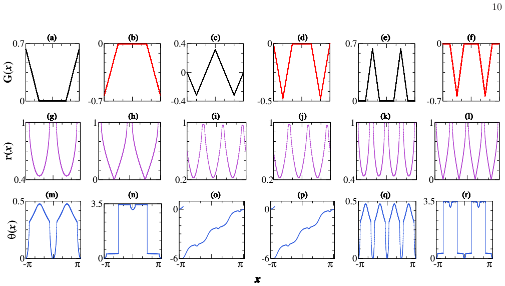
are also shown with brown tri- angles. The plots are presented for G(x) where repulsive coupling is present in combination with attractive or null coupling regions. From Fig. 4 we observe that the ana- lytical and numerical solutions match well in the α range where synchronized solutions (or SS ) exist. The form of G(x) and the phase profile of the system ...
-
[10]
Inter- estingly, the two antiphase clusters in AP C2 move with time; however, the rate of their movement depends upon the initial condition from which they have evolved. To probe further into the switching of in-phase chimera to antiphase chimera, we make the attractive coupling repulsive in a probabilistic manner by introducing repul- sive connections wi...
-
[11]
The subfigures in the top panel show the variation of fsync with p when the re- pulsive connections are introduced only in the attractive coupling region (keeping the neutral coupling region un- changed). We observe that as the repulsive connections increase, indicated by an increase in p, the number of synchronised oscillators in IP C2 first decreases, res...
-
[12]
From the plots, we observe that when the repulsive interactions are introduced in the en- tire range, IP C2 and AP C2 collapse to a desynchronized state (Fig. 10(c),(d)). The coupling function G(x), and the corresponding asymptotic phase distribution of the system at p = 0 and p = 1 are shown in the insets. Therefore, from Fig. 10 we conclude that the tra...
-
[13]
The results for G(x) resulting in 4 and 6 cluster chimeras are shown in Fig
The attractive coupling kernel G(x), which leads to antiphase chimeras with an even number of clusters, gives rise to a fully desynchronized state when the positive (attrac- tive) coupling region becomes negative (repulsive). The results for G(x) resulting in 4 and 6 cluster chimeras are shown in Fig. 14. From our investigation on the multi-cluster chimer...
-
[14]
we get, ∂q ∂t = − iωq + i 2 [ Re− iβ + ¯Reiβ q2] . (20) The order parameter can be written as, R(x, t ) = ∫ π − π ∫ ∞ −∞ G(x − x′)g(ω )q(x′, ω, t )dωdx ′. (21) 11 Assuming that ω is taken from a Lorentzian distri- bution with half-width-at-half-maxima and centre of the distribution as D and ω o respectively such that, g(ω ) = D/π (ω − ω o)2 + D2 . (22) We...
- [15]
- [16]
- [17]
-
[18]
E. L. Schwartz, Computational neuroscience (MIT Press, 1993)
work page 1993
- [19]
-
[20]
A. Gir´ on, H. Saiz, F. S. Bacelar, Roberto F. S. Andrade, and J. G´ omez-Garde˜ nes,Chaos 26, 065302 (2016)
work page 2016
-
[21]
B. Paul, B. Bandyopadhyay, and T. Banerjee, Phys. Rev. E 110, 034210 (2024)
work page 2024
-
[22]
S. H. Strogatz and I. Stewart, Sci. Am. 269, 102 (1993)
work page 1993
-
[23]
S. H. Strogatz and R. E. Mirollo, Phys. Rev. E 47, 220 (1993)
work page 1993
- [24]
-
[25]
Y. Kuramoto and D. Battogtokh, Nonlinear Phenom. Complex Syst. 5, 380–385 (2002)
work page 2002
-
[26]
D. M. Abrams and S. H. Strogatz, Phys. Rev. Lett. 93, 174102 (2004)
work page 2004
-
[27]
M. J. Panaggio and D. M. Abrams, Nonlinearity 28, R67 (2015)
work page 2015
-
[28]
N. C. Rattenborg, C. J. Amlaner, and S. L. Lima, Neurosci. Biobehav. Rev. 24, 817 (2000)
work page 2000
-
[29]
S. W. Haugland, J. Phys. Complex. 2, 032001 (2021)
work page 2021
-
[30]
C. G. Mathews, J. A. Lesku, S. L. Lima, and C. J. Am- laner, Ethology 112, 286 (2006)
work page 2006
- [31]
- [32]
-
[33]
T. Makinwa, K. Inaba, T. Inagaki, Y. Yamada et al. , Commun. Phys. 6, 121 (2023)
work page 2023
-
[34]
E. M. Cherry and F. H. Fenton, New J. Phys. 10, 125016 (2008)
work page 2008
-
[35]
E. A. Martens, S. Thutupalli, A. Fourri` ere, and O. Hal- latschek, Proc. Natl. Acad. Sci. USA 110, 10563 (2013)
work page 2013
-
[36]
P. Ebrahimzadeh, M. Schiek, and Y. Maistrenko, Chaos 32, 103118 (2022)
work page 2022
-
[37]
M. R. Tinsley, S. Nkomo, and K. Showalter, Nat. Phys. 8, 662–665 (2012)
work page 2012
-
[38]
M. H. Matheny, J. Emenheiser, W. Fon, A. Chapman et al., Science 363, eaav7932 (2019)
work page 2019
-
[39]
J. C. Gonz´ alez-Avella, M. G. Cosenza, and M. San Miguel, Physica A 399, 24 (2014)
work page 2014
-
[40]
I. Omelchenko, O. E. Omel’chenko, P. H¨ ovel, and E. Sch¨ oll,Phys. Rev. Lett. 110, 224101 (2013)
work page 2013
-
[41]
S. R. Ujjwal and R. Ramaswamy, Phys. Rev. E 88, 032902 (2013)
work page 2013
-
[42]
K. Sathiyadevi, V. K. Chandrasekar, D. V. Senthilkumar , and M. Lakshmanan, Phys. Rev. E 97, 032207 (2018)
work page 2018
-
[43]
G. B. Ermentrout and N. Kopell, SIAM J. Appl. Math. 54, 478 (1994)
work page 1994
- [44]
- [45]
-
[46]
A. Hutt, M. Bestehorn, and T. Wennekers, Netw., Comput. Neural Syst. 14, 351 (2003)
work page 2003
-
[47]
R. Zillmer, R. Livi, A. Politi, and A. Torcini, Phys. Rev. E 74, 036203 (2006)
work page 2006
-
[48]
D. W. Jordan and P. Smith, Nonlinear Ordinary Differ- ential Equations, Oxford University Press, (2007)
work page 2007
- [49]
- [50]
-
[51]
C. R. Laing, Physica D 238, 1596 (2009)
work page 2009
-
[52]
S. Gharsalli, R. Aloui, S. Mhatli, A. Corona-Chavez et al., Prog. Electromagn. Res. B 116, 33–47 (2026)
work page 2026
-
[53]
P. H. Tiesinga and T. J. Sejnowski, Front. Human Neurosci. 4, 196 (2010)
work page 2010
-
[54]
S. E. Qasim, I. Fried, and J. Jacobs, Cell 184, 3242 (2021)
work page 2021
-
[55]
M. J. Sedghizadeh, H. Aghajan, Z. Vahabi, S. N. Fatemi, and A. Afzal, Brain Struct. Funct. 227, 2957 (2022)
work page 2022
- [56]
-
[57]
S. R. Ujjwal, N. Punetha, and R. Ramaswamy, Phys. Rev. E 93, 012207 (2016)
work page 2016
-
[58]
Z. Cai, Z. Liu, S. Guan, J. Kurths, and Y. Zou, Phys. Rev. Lett. 133, 227201 (2024)
work page 2024
discussion (0)
Sign in with ORCID, Apple, or X to comment. Anyone can read and Pith papers without signing in.