Taking rational numbers at random

Nicola Cufaro Petroni

Taking rational numbers at random

T0 review · 0 major / 5 minor · reviewed 2026-08-14 · deepseek-v4-flash

Challenge this review Re-run · record.json Download PDF Read on arXiv ↗ Review JSON

Pith's one-line read Rationals in $[0,1]$ admit a limiting equiprobable draw: single points get probability zero, intervals get their length.

desk verdict Correct but elementary: the main limit theorem is a standard triangular-array weak convergence result, delivered cleanly but with two sloppy example conditions and a missed totient identity in Section 7. read the letter →

arxiv 1908.06944 v1 pith:Z4Q5UMZ6 submitted 2019-08-19 math.PR

Nicola Cufaro Petroni This is my paper · ORCID

classification math.PR MSC 60A0560B1060E05

keywords rationalnumbersasymptoticequiprobabilitydiscretedistributionsuniformdistributioncountableadditivityrandomdenominatorintervalprobabilities

verification ladder T0 review T1 audit T2 compute T3 formal

The pith

A machine-rendered reading of the paper's core claim, the machinery that carries it, and where it could break.

The reading

The paper asks what it could mean to choose a rational number in $[0,1]$ uniformly at random, and argues that a precise asymptotic answer exists. Because no exact uniform distribution can live on the countable set $\mathbb{Q}_0$ under ordinary countably additive probability, the paper builds distributions on $\mathbb{Q}_0$ by choosing a denominator $M$ and then an equiprobable numerator $N$ from $0$ to $M$. It proves that when the denominator law is flattened in a controlled way, the probability of every single rational tends to $0$ while the probability of falling in an interval $(a,b]$ tends to $b-a$. In that limit the rationals in $[0,1]$ behave like a uniform draw, which is the paper's sense of taking rationals at random.

What carries the argument

The load-bearing device is representing the random rational as a ratio $Q=N/M$, where $M$ selects a denominator and $N$ is conditionally uniform on $\{0,1,\ldots,M\}$. For a fixed irreducible $q=n/m$, the probability of $q$ is the sum over all multiples $\ell$ of the denominator $m$ of $P\{M=\ell m\}/(\ell m+1)$; the proof controls this sum by the expectation $\mu_k=E[1/M_k]$. The flattening condition $s_k\ln k\to 0$ forces $\mu_k\to 0$ through the harmonic-number bound, and this single decay estimate is what makes atom probabilities vanish and interval probabilities converge to $b-a$. Floor-function identities then write interval probabilities and the cdf as sums over $M$ that are squeezed between $b-a$ and $b-a$ plus a multiple of $\mu_k$.

What would settle it

Take denominators uniform on $\{1,\ldots,k\}$ and compute, for a fixed rational $q=n/m$, the exact atom probability $(1/k)\sum_{\ell=1}^{\lfloor k/m\rfloor}1/(\ell m+1)$; the claim fails if this does not tend to $0$ as $k\to\infty$. Similarly, for a fixed interval $(a,b]$, the finite floor-sum expression for $P\{a<Q\le b\}$ must tend to $b-a$, and a numerical check at $k=10^5$ is already shown in the paper.

Watch

Extended reading notes

Core claim

Under the construction $Q=N/M$, with $P\{N=n\mid M=m\}=1/(m+1)$ and denominator distributions $p_m(k)$ whose supremum $s_k$ satisfies $s_k\ln k\to 0$, the paper proves in Proposition 5.2 that $P_k\{Q=q\}\to 0$ for each $q\in\mathbb{Q}_0$ and $P_k\{a<Q\le b\}\to b-a$ for $0\le a<b\le 1$; the cdf converges pointwise to the uniform cdf. The paper stresses that this does not manufacture a uniform distribution on $\mathbb{Q}_0$, because that would violate countable additivity; it is an asymptotic equiprobability in which each rational's individual probability dies out while rationals pooled in any interval carry exactly the interval's length. The variance of $Q$ also converges to $1/12$, matching the uniform law on $[0,1]$.

Load-bearing premise

The whole setup leans on the standard rule that probabilities add up over countably many disjoint events; under that rule no uniform distribution on the rationals can exist, and the asymptotic limit is the only route offered.

Editorial extensions

If this is right

For any denominator sequence meeting $s_k\ln k\to0$ — finite uniform, geometric with $w\to0$, or Poisson with $\lambda\to\infty$ — the rational-valued variable converges in distribution to the uniform law on $[0,1]$.
A practical simulation with large fixed $k$ and equiprobable denominators $1,\ldots,k$ gives a sample whose bin frequencies are almost uniform on $[0,1]$, although only finitely many rationals receive positive probability at that finite stage.
There is no contradiction with the impossibility of an exact uniform distribution: the limiting measure is the Lebesgue uniform law on $[0,1]$, not a measure supported on $\mathbb{Q}_0$.
The variance formula $V[Q]=1/12+\mu_k/6$ gives a quantitative, finite-$k$ check of how close the draw is to uniformity.

Reading between the lines

Editorial extensions of the paper, not claims the author makes directly.

The proof only uses the harmonic bound to force $\mu_k=E[1/M_k]\to0$, so the essential hypothesis is likely that $E[1/M_k]\to0$; the condition $s_k\ln k\to0$ is a sufficient but probably not necessary route to it.
If one dropped countable additivity and allowed finitely additive probabilities, an exact uniform distribution on $\mathbb{Q}_0$ would exist; the paper's impossibility claim would fail, while its interval-limit result would survive as an approximation theorem for that nonstandard uniform law.
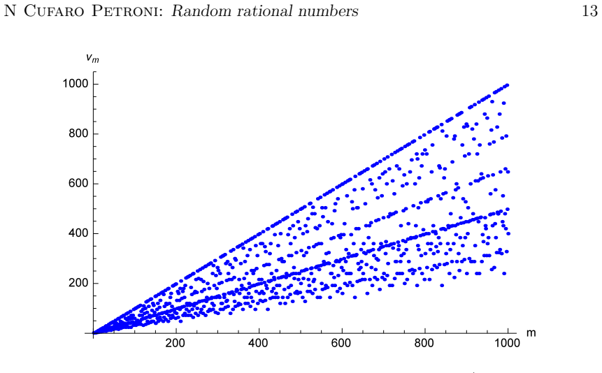
Connecting the paper's asymptotic-uniform rational draws to the irregular counting function $\nu_m$ could lead to distributions that weight reduced fractions directly, which the paper leaves open.

Share X Bluesky LinkedIn Reddit HN

Signed reviews

No signed human review yet.

Editorial analysis

A structured set of objections, weighed in public.

Desk editor's note, referee report, and a circularity audit.

Desk Editor's Note

read the letter

The core thing to know: the mathematical result is right, the proof is straightforward and readable, but the paper's novelty is modest and it has a few fixable factual slips. If you referee it, treat it as a solid pedagogical note, not a research breakthrough.

What is actually good: the construction is clean. You take a sequence of denominator distributions, assume conditionally uniform numerators, and show under a uniform-flattening condition (s_k ln k → 0) that each rational's point mass goes to zero while interval probabilities go to b−a. Lemma 5.1 and Proposition 5.2 are correct; the floor-function sandwich works, and the countable-additivity issue is handled explicitly. Formula (10), the point mass as a sum over multiples of the irreducible denominator, is a nice closed form. The paper also honestly notes that no exact uniform distribution on Q0 exists, which is the right framing.

Soft spots, in order of significance. First, the examples overclaim. The geometric case is said to satisfy (13) whenever w_k → 0, but the condition really needs w_k ln k → 0. Similarly, the Poisson case is said to work for λ_k → ∞, but you need λ_k/(ln k)^2 → ∞. These are easy fixes, but as written the examples are wrong. Second, Section 7 says ν_m has no closed form and that sequencing Q0 is largely open, but for m ≥ 2, ν_m is just Euler's totient φ(m), and complete enumeration schemes already exist (Farey sequences, Stern–Brocot, Calkin–Wilf). The paper's coefficient-matching trick to compute ν_m is a neat exercise, but presenting it as an open problem is misleading. Third, the philosophical point about countable additivity is fine, but the paper could acknowledge that finitely additive uniform distributions would change the conclusion; this is a framing remark, not a flaw in the math.

None of this threatens the central theorem. The proof of Proposition 5.2 is sound, and the flaws are peripheral. The paper is exactly what it looks like: a clear, elementary demonstration that rationals can be asymptotically equiprobable in a weak-convergence sense. It does not resolve any open problem, and the result is a special case of standard triangular-array theory, but it is a useful reference for teaching and for anyone who wants a concrete example.

I would send it to peer review with a light touch: correct the example conditions, add the φ(m) observation, and downscope the claims about sequencing. That is a revision, not a rejection. The paper deserves a serious referee because it is genuinely clear and mostly correct.

Referee Report

0 major / 5 minor

Summary. The paper proposes a way to assign probabilities to rational numbers in [0,1] by writing Q=N/M, giving M a distribution on the positive integers and, conditional on M=m, taking N uniform on {0,...,m}. The probability of a rational q with irreducible denominator j is then a sum over ℓ of P(M=ℓj)/(ℓj+1). The paper shows that no exact uniform distribution on Q0 exists in the standard countably additive framework, and proves (Proposition 5.2) that for a sequence of denominator laws whose maximal atom s_k satisfies s_k ln k→0, all point probabilities vanish while P(a<Q≤b)→b−a, so the law becomes asymptotically uniform on [0,1]. Examples, closed-form formulas for geometric denominators, a simulation-oriented finite-support construction, and a discussion of sequencing Q0 are included.

Significance. If it holds, the paper gives a clean rigorous sense in which rational numbers in [0,1] can be drawn 'almost uniformly', despite the nonexistence of an exact uniform distribution on a countable set. The construction contains no fitted parameters, and the main derivation is elementary and correct: Lemma 5.1 and Proposition 5.2 are proved by explicit floor-function bounds, and the countable-additivity obstruction in Section 2 is handled honestly. The paper is modest in scope but self-contained, and its central claim is not circular: condition (13) is a genuine hypothesis on the denominator laws. The main weaknesses are local presentation issues in the examples and in the sequencing remarks.

minor comments (5)

[Section 5, examples after (13)] For the geometric family, condition (13) requires w_k ln k→0, and for the Poisson family it requires λ_k/(ln k)^2→∞. The text says only that w_k is infinitesimal and λ_k is divergent, which is not sufficient; for instance w_k=1/ln k or λ_k=ln k satisfies those weaker statements but violates (13). Please state the correct rate conditions explicitly.
[Lemma 5.1] The assertion that R_k is an infinitesimal remainder is correct but not justified in the proof. It follows immediately because for m>k one has 1/m≤1/k, so R_k≤(1/k)∑_{m>k}p_m(k)≤1/k; adding this one-line argument would make the proof complete.
[Proposition 5.2, proof of (16)] The displayed inequality x−xμ_k < F_Q(x) < x+(1−x)μ_k is not strictly true at x=1, where F_Q(1)=1 and the right-hand side equals 1. Use non-strict inequalities or restrict the displayed line to 0≤x<1 and handle x=1 separately.
[Section 7, Eq. (19)] The coefficient comparison gives ∑_{d|r}ν_d = r, which means ν_m is exactly Euler's totient φ(m) for m≥2. Identifying ν_m with φ(m) would connect the sequencing discussion to standard number-theoretic facts and simplify the recursive computation. The displayed lines such as 'ν_1/3+ν_2/3=1' are also confusing; they should be phrased as coefficients of powers of z, e.g. (ν_1+ν_2)/3=1 for z^3.
[Section 6.1, Figure 1] The caption lists fixed values (0.9, 0.5, 0.1, 0.01, 0.001) of w, while Proposition 5.2 concerns a sequence w_k→0. The figure is illustrative, but the text should state explicitly that it does not by itself demonstrate the rate condition (13).

Circularity Check

0 steps flagged · score 0.0 of 10

No significant circularity identified.

full rationale

The paper's central result, Proposition 5.2 with equations (15) and (16), is a proved limit theorem rather than a repackaged input. The construction begins by defining Q=N/M with N conditionally uniform on {0,...,M}, and then imposes the flattening condition sup_m p_m(k) ln k -> 0 on the sequence of denominator distributions. This condition is an explicit hypothesis, not a conclusion or a fitted parameter. The interval-probability limit b-a is derived through floor-function bounds and Lemma 5.1; it is not assumed by the construction. No fitted quantity is later relabeled as a prediction, and the theorem does not rely on any self-citation: the only citation is to a standard reference for harmonic and hypergeometric series. The countable-additivity limitation discussed in Section 2 frames the problem but is not used as a premise in the proof of the asymptotic result. The peripheral issues in the geometric and Poisson examples—where the stated sufficient conditions are weaker than condition (13)—are mathematical or expository caveats, not circularity. Overall, the derivation is self-contained and the limit theorem has genuine mathematical content.

Assumptions & free parameters 4 free parameters · 5 assumptions · 0 invented entities

The central proof has no fitted parameters: the denominator sequence p_m(k) is a hand-chosen modeling device and the theorem states a sufficient condition. The main axioms are countable additivity and standard analytic estimates. No invented entities are introduced.

free parameters (4)

Denominator distribution p_m(k)
Defines the construction; any sequence satisfying sup_m p_m(k) ln k →0 works. It is chosen by hand, not fitted to data.
Geometric rate w_k
Example in Section 6.1: p_m(k)=w_k(1-w_k)^{m-1} with w_k→0 fast enough; a tuning constant, not fitted.
Poisson rate λ_k
Example in Sections 5 and 6.2: must diverge fast enough that s_k ln k→0, i.e. λ_k/(ln k)^2→∞; the paper only says λ_k→∞, which is insufficient.
Finite support size k
Example in Section 6.2: p_m(k)=1/k for m=1..k; a tuning parameter for the approximation, not fitted.

assumptions (5)

domain assumption Probability measures are countably additive; a legitimate distribution on Q0 must have P(Q=q) summing to 1 over all q.
Section 2: continuous cdfs on Q0 violate countable additivity because Q0 is a countable union of singletons.
standard math Every rational q∈[0,1] has a unique irreducible representation q=n/m with gcd(n,m)=1.
Equation (1) sums over all representations ℓn/ℓm, relying on uniqueness of the reduced form.
standard math The harmonic numbers H_k grow as ln k and the tail mass of each probability distribution tends to 0.
Lemma 5.1 uses these to prove μ_k=E[1/M_k]→0 under (13).
standard math All series with non-negative terms may be rearranged and bounded termwise.
Equations (5), (6), (10), and (12) exchange sums freely; Tonelli's theorem justifies this.
standard math Power series are uniquely determined by their coefficients.
Section 7 equates coefficients in equation (19) to compute ν_m recursively.

how reviews work

0 comments

Cite this review

Pith. "Pith review of Taking rational numbers at random." pith.science (2026). https://pith.science/paper/Z4Q5UMZ6

@misc{pith2026190806944,
  author       = {Pith},
  title        = {Pith review of: Taking rational numbers at random},
  year         = {2026},
  howpublished = {\url{https://pith.science/paper/Z4Q5UMZ6}},
  note         = {Machine review of arXiv:1908.06944}
}

abstract

We outline some simple prescriptions to define a distribution on the set $\mathbb{Q}_0$ of all the rational numbers in $[0,1]$, and we then explore both a few properties of these distributions, and the possibility of making these rational numbers asymptotically equiprobable in a suitable sense. In particular it will be shown that in the said limit -- albeit no uniform distribution can be properly defined on $\mathbb{Q}_0$ -- the probability allotted to a single $q\in\mathbb{Q}_0$ asymptotically vanishes, while that of the subset of $\mathbb{Q}_0$ falling in an interval $[a,b]$ goes to $b-a$. We finally give some hints to completely sequencing without repetitions the numbers in $\mathbb{Q}_0$ as a prerequisite to the laying down of more distributions on it

Figures

Figures reproduced from arXiv: 1908.06944 by the authors.

**Figure 2.** Numerosity νm of the different rational numbers q .= n/m sharing a common, irreducible denominator m we find instead X∞ m=1 Xm n=0 w(1 − w) m−1 m + 1 2F1 [PITH_FULL_IMAGE:figures/full_fig_p013_2.png] view at source ↗

**Figure 3.** Typical histogram of the relative frequencies of a sample o [PITH_FULL_IMAGE:figures/full_fig_p015_3.png] view at source ↗

Discussion (0). Continue with ORCID to comment.

Reference graph

Works this paper leans on

35 extracted references · 35 canonical work pages

[1]

I.S.\ Gradshteyn and I.M.\ Ryzhik, Table of Integrals, Series and Products (Academic Press, Burlington 2007 )

work page 2007
[2]

M.\ Abramowitz and I.\ A.\ Stegun Handbook of Mathematical Functions

work page
[3]

J.\ Bertrand, Calcul des

work page
[4]

Gnedenko, The Theory of Probability (MIR, Moscow 1978)

B.V. Gnedenko, The Theory of Probability (MIR, Moscow 1978)

work page 1978
[5]

A.M.\ Mathai, An Introduction to Geometrical

work page
[6]

A.\ Papoulis and S.U.\ Pillai, Probability, Random Variables and Stochastic Processes (McGraw-Hill, Boston 2002)

work page 2002
[7]

E.\ Czuber, Wahrscheinlichkeitsrechnung und ihre Anwendungen auf Fehlerausgleichung, Statistik und

work page
[8]

Wiley&Sons, New York 1990)

B.\ De Finetti, Theory of Probability (J. Wiley&Sons, New York 1990)

work page 1990

Show all 35 references

[9]

A.N.\ Shiryayev, Probability (Springer, New York 1984)

1984
[10]

M.\ Lo\`eve, Probability Theory I--II (Springer,
[11]

J.\ Cicho\'n, Z.\ Go e biewski , DMTCS Proc
[12]

T.M.\ Cover, J.M.\ Thomas, Elements of Information
[13]

Gintautas, M.I.\ Ham,

L.M.A.\ Bettencourt, V. Gintautas, M.I.\ Ham,
[14]

C.\ Tsallis, J.\ Stat.\ Phys.\ 52 (1988) 479

1988
[15]

C.W.\ Gardiner, Handbook of stochastic
[16]

N.\ Cufaro Petroni and M.\ Pusterla, Physica A 388 (2009)

2009
[17]

P.\ Garbaczewski, J.\ R.\ Klauder and R.\ Olkiewicz, Phys.\ Rev.\
[18]

N.\ Laskin, Phys.\ Rev.\ E 62 (2000) 3135.\\

2000
[19]

R.\ Gorenflo and F.\ Mainardi Frac.\ Calc.\
[20]

N.\ Cufaro Petroni, (2010) arXiv:1006.1833v1 [math.PR]

2010 arXiv
[21]

K.\ Sato: L\'evy processes and infinitely
[22]

D.\ Applebaum: L processes and Stochastic Calculus
[23]

N.\ Cufaro Petroni, Physica A 387 (2008)

2008
[24]

N.\ Cufaro Petroni, J.\ Phys.\ A 40 (2007)

2007
[25]

C.\ Berg and C.\ Vignat, J.\ Phys.\ A 41 (2008) 265004

2008
[26]

C.\ C.\ Heyde and N.\ N.\ Leonenko, Adv.\ Appl.\ Prob.\
[27]

W.\ Feller, An introduction to probability theory and its
[28]

N.\ Balakrishnan and V.\ B.\ Nevzorov,
[29]

W,\ Rudin, Functional analysis (McGraw-Hill, New York, 1973)

1973
[30]

D.\ W.\ Stroock, An introduction to partial
[31]

D.\ W.\ Stroock and S.\ R.\ S.\ Varadhan,
[32]

E.\ Madelung, Z.\ Physik 40 (1926) 332

1926
[33]

A.\ Vivoli, C.\ Benedetti and G.\ Turchetti,
[34]

W.\ Paul and J.\ Baschnagel Stochastic processes: from physics
[35]

Ph.\ E.\ Protter, Stochastic integration and

Pith tools

Reviewed August 14, 2026 · model on record in the stance chip above.

[1] [1]

I.S.\ Gradshteyn and I.M.\ Ryzhik, Table of Integrals, Series and Products (Academic Press, Burlington 2007 )

work page 2007

[2] [2]

M.\ Abramowitz and I.\ A.\ Stegun Handbook of Mathematical Functions

work page

[3] [3]

J.\ Bertrand, Calcul des

work page

[4] [4]

Gnedenko, The Theory of Probability (MIR, Moscow 1978)

B.V. Gnedenko, The Theory of Probability (MIR, Moscow 1978)

work page 1978

[5] [5]

A.M.\ Mathai, An Introduction to Geometrical

work page

[6] [6]

A.\ Papoulis and S.U.\ Pillai, Probability, Random Variables and Stochastic Processes (McGraw-Hill, Boston 2002)

work page 2002

[7] [7]

E.\ Czuber, Wahrscheinlichkeitsrechnung und ihre Anwendungen auf Fehlerausgleichung, Statistik und

work page

[8] [8]

Wiley&Sons, New York 1990)

B.\ De Finetti, Theory of Probability (J. Wiley&Sons, New York 1990)

work page 1990