REVIEW 4 major objections 4 minor 35 references
Bayesian Spatial Field Reconstruction with Unknown Distortions in Sensor Networks
T0 review · 4 major / 4 minor · reviewed 2026-08-14 · deepseek-v4-flash
Pith's one-line read Unknown affine sensor distortions can be inferred jointly with the spatial field, giving a closed-form best linear unbiased estimator and empirical-Bayes reconstructions nearly as accurate as knowing the distortions exactly.
desk verdict Solid extension of the authors' earlier mixture-GP work, with one real covariance typo and an evaluation that stays inside the model's own prior; worth a serious referee, not acceptance as-is. read the letter →
The pith
A machine-rendered reading of the paper's core claim, the machinery that carries it, and where it could break.
The reading
What carries the argument
The engine of the paper is the affine distortion mixture: each sensor's observation is $y_{n,m}=a_n(f(x_n)+\epsilon_{n,m})+b_n$ with $\epsilon_{n,m}\sim N(0,\varsigma^2)$, and $(a_n,b_n)$ follows a finite mixture prior $\pi(\psi_n)=q_n^{(0)}\delta_{(1,0)}+\sum_{k=1}^K q_n^{(k)}\pi_k(\psi_n)$ that includes an atom at no distortion. Theorems 1 and 2 show that, conditional on $\psi$, the sufficient statistics $(g_n,s_n)=(\sum_m y_{n,m},\sum_m y_{n,m}^2)$ leave the field and distortion parameters in a joint Gaussian form, so the posterior of $\psi$ and the predictive of $f_*$ are explicit up to the normalizing constant. Theorem 3 converts those moment expressions into S-BLUE, whose weights require only the prior moments $\mathbb{E}[a]$, $\mathbb{E}[b]$, $\mathbb{E}[aa^\top]$, $\mathbb{E}[bb^\top]$, $\mathbb{E}[ab^\top]$; this is what makes the online estimate a single $O(N)$ linear combination after an offline $O(N^3)$ inversion. The two empirical-Bayes optimizers, CEM and ICM, are the tools that replace the intractable posterior average by a point estimate $\hat\psi$.
What would settle it
Simulate a sensor network in which a known fraction of sensors have nonlinear or time-varying distortions (for example, gain that drifts linearly over time), generated independently of the assumed mixture prior, then run S-BLUE and the empirical-Bayes estimators on these data; if the reconstruction error degrades substantially relative to the oracle while the same methods perform well under affine distortions, the model's robustness claim is falsified.
Extended reading notes
Core claim
The central claim is that, in the mixture-of-Gaussian-process-expert model with affine gain-offset distortions, everything needed for spatial reconstruction is computable in closed form except the normalizing constant of the posterior over distortions. Theorem 1 gives the log-posterior of the distortion parameters $\psi=(\psi_n)_{n=1:N}$; Theorem 2 gives the posterior predictive $p(f_*|y)$ as a Gaussian-mixture integral whose integrand $p(f_*|y,\psi)$ is Gaussian. Theorem 3 then shows the Spatial Best Linear Unbiased Estimator (S-BLUE), restricted to estimators linear in the per-sensor sample means $\bar{g}=M^{-1}g$, has the closed form $\hat h(y)=\mu_* + \mathrm{Cov}[\bar{g},f_*]^\top \mathrm{Cov}[\bar{g}]^{-1}(\bar{g}-\mathbb{E}[\bar{g}])$, with all moments evaluated from the mixture prior. For nonlinear estimation, the paper computes a MAP estimate of $\psi$ by cross-entropy or iterated conditional modes and plugs it into the Gaussian predictive, calling this empirical Bayes. The paper's experiments, including a real temperature dataset with synthetic distortions, show these estimators track the oracle that knows the distortions and beat the naive estimator that ignores them.
Load-bearing premise
The load-bearing premise is that every sensor's distortion is exactly a simple 'scale then add' map, $u\mapsto a_n u+b_n$, with $(a_n,b_n)$ drawn from a known finite mixture that includes an atom at no distortion; nonlinear, drifting, or otherwise unanticipated faults are not covered by the model.
Editorial extensions
If this is right
- A fusion center can reconstruct the field at arbitrary locations without knowing which sensors are faulty, provided the affine-mixture prior is correct; per-sensor distortion parameters are estimated implicitly or explicitly.
- S-BLUE needs no online optimization: after an offline $O(N^3)$ preparation, the online update is $O(N)$, making real-time field reconstruction feasible for large networks.
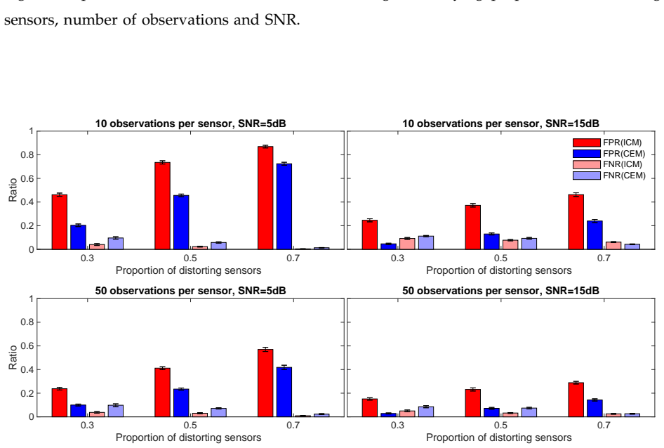
- The empirical-Bayes estimators recover most of the oracle performance when observations per sensor and SNR are sufficiently high, but with scarce data they can misclassify all sensors as distorting, and at very high SNR both optimizers degrade as the paper's Remark 4 notes.
- Distributed versions improve scalability and, in high-SNR settings, can beat the centralized empirical-Bayes estimators because lower-dimensional optimization is easier.
- The method detects distorting sensors with low false-positive and false-negative rates when SNR and sample size are adequate, and reconstruction quality degrades only mildly as the proportion of distorting sensors grows, unlike the naive baseline.
Reading between the lines
- A natural by-product of the mixture prior is a per-sensor fault score: the posterior probability that $Z_n=0$ (no distortion) is exactly the quantity behind the paper's false-positive and false-negative rates, and could be surfaced to a network operator as a reliability flag without extra computation.
- Because S-BLUE uses only prior moments, it cannot adapt to the actual distortions; a cheap hybrid policy would run S-BLUE online as a safe default and switch to an empirical-Bayes estimate once enough observations per sensor accumulate.
- The paper's Remark 4, that very high SNR makes both optimizers degrade, suggests the posterior mode becomes ill-posed when the likelihood is extremely concentrated; a testable fix is to replace the point estimate $\hat\psi$ with a Laplace approximation or a few posterior samples.
- The same affine-distortion plus Gaussian-field template applies to other calibration-inverse problems, such as reconstructing pollutant or radio-frequency fields from crowdsourced sensors, where the gain-offset model is already common.
Signed reviews
Editorial analysis
A structured set of objections, weighed in public.
Referee Report
Summary. The paper develops a Bayesian framework for reconstructing a Gaussian-process spatial field from sensor readings that are subject to unknown affine distortions (gain and offset), modeled by a finite mixture prior with an atom at no distortion. It derives the posterior over distortion parameters (Theorem 1), the posterior predictive distribution (Theorem 2), a closed-form Spatial Best Linear Unbiased Estimator (Theorem 3), and empirical-Bayes estimators whose MAP distortion estimates are obtained by Cross-Entropy (CEM) and Iterated Conditional Modes (ICM), together with distributed variants. Experiments on synthetic fields and on US EPA temperature data with simulated distortions compare S-BLUE, CEM, and ICM against oracle and naive baselines. The paper claims that the proposed methods reconstruct the field with materially lower MSE than the naive baseline and close to the oracle in the tested settings.
Significance. If corrected, the paper is a useful practical contribution: it provides a closed-form linear estimator with a clean offline/online complexity split, tractable empirical-Bayes alternatives, and distributed versions, and the derivations of Theorems 1 and 2 appear sound. The computational complexity analysis is careful and the experimental comparison is reasonably extensive. However, the central theorem contains an algebraic error, the CEM objective and the ICM pseudocode have inconsistencies, and the experimental validation only exercises the exact generative distortion model. These issues are fixable, and the main claims are plausible conditional on those fixes; the paper's contribution is an estimation scheme for a specific and well-motivated distortion model rather than a fundamentally new statistical methodology.
major comments (4)
- [§IV, Theorem 3, Eq. (19); Appendix A-C, Eq. (43)] Equation (19) writes the cross-covariance contribution to Cov[g_bar] as diag(mu)(E[ab^T] + E[ab^T]^T). Expanding Cov(A mu + b) gives diag(mu) E[ab^T] + E[ab^T]^T diag(mu), not diag(mu)(E[ab^T] + E[ab^T]^T). The two expressions coincide only when diag(mu) commutes with E[ab^T], which holds for a constant prior mean; all experiments in the paper use a constant prior mean, so the numerical results are not directly affected, but the theorem as stated is incorrect and must be corrected before publication.
- [§V-A, CEM objective after Eq. (22)] The CEM section defines the objective as J(psi) = log p(psi|y) + log pi(psi). Since log p(psi|y) in Theorem 1 already contains the term +log pi(psi), this definition double-counts the prior and is not the MAP objective of Eq. (22). As written, Algorithm 2 would maximize log p(y|psi) + 2 log pi(psi) up to constants. The authors should either define J(psi) = log p(y|psi) + log pi(psi) or explicitly state that the expression denoted p(psi|y) in the CEM section is the unnormalized likelihood contribution only.
- [§V-B, Algorithm 4 (ICM)] The quantities nu_n and zeta_n in Eqs. (25)-(26) depend on psi_{(-n)} through g_tilde_{(-n)}, but the pseudocode computes them once in Lines 2-3 before the repeat loop and never recomputes them after each coordinate update. Without recomputation, the algorithm is not the iterated conditional-mode algorithm described in the text, and the claim that it converges to a conditional mode is unsupported. The authors should move the computation of nu_n and zeta_n inside the repeat loop and update the complexity analysis accordingly, or explain why no update is needed.
- [§VII and §VIII, experimental validation] All simulated distortions, in both the synthetic experiments and the real-data experiment, are generated from the exact affine mixture prior specified in A4/P4, and the real-data "ground truth" is itself a posterior sample from the fitted GP. The paper therefore demonstrates self-consistency under the model but not robustness to distortion families outside the assumed class, such as saturation, deadband, clipping, time-varying gain, or component densities different from the prior. I recommend adding misspecification experiments of this kind, or explicitly limiting the robustness claims to the affine mixture family.
minor comments (4)
- [Algorithm 3, E-step] The displayed formula for Q(theta; theta_t) is missing the logarithm: it should read Q(theta; theta_t) = sum_s sum_k p[s]_k log p(psi[s] | z[s]=k; theta), as the surrounding text correctly states.
- [Abstract and Conclusion] There are typographical errors: "W e" in the abstract and "preformed" in the conclusion should be corrected.
- [Algorithm 2] The termination condition for the CEM algorithm is not specified; a concrete stopping rule, such as a threshold on the relative change of J or on the change of the sampling distribution parameters, would make the algorithm reproducible.
- [§VIII-C] The replication protocol for the real-data experiment is not fully clear: it should state explicitly whether the distortion parameters are re-drawn for each of the 20 days or fixed across days, and how many noise realizations are averaged for each reported MSE.
Circularity Check
Derivation chain is self-contained; the in-model evaluation is a validation limitation, not circularity.
full rationale
Walking the claimed derivation chain: Theorem 1 marginalizes the GP latent values in a linear-Gaussian model, Theorem 2 applies standard conditional Gaussian identities and integrates over the parameter posterior, and Theorem 3 minimizes the explicit Bayes risk over the linear family, with all required moments evaluated directly from the stated mixture prior in Eqs. (17)-(19) and (40)-(45). The empirical Bayes estimators in Section V explicitly define psi-hat as the maximizer of log p(psi|y) in Eq. (22) and then plug it into the conditional predictive distribution; no fitted parameter is renamed as a new prediction. The distributed fusion rules are convex combinations chosen by the stated risk criteria, not by assuming the conclusion. Self-citations such as [1], [24], [25], and [28] are used as background for Gaussian-process sensor-network modeling; the distortion mixture model itself is fully specified in the paper (A4, P3-P4) rather than imported as an unverified black box. The semi-synthetic real-data experiment does generate ground truth from a posterior sample of the fitted GP and draws simulated distortions from the assumed prior, so the evaluation is in-model; this is an external-validity limitation, but it is not a circular step in the derivation chain.
Assumptions & free parameters
free parameters (7)
- GP hyperparameters (signal mean, signal std, noise std, length-scale) =
signal mean 30.5034 C, signal std 4.6587 C, noise std 1.6340 C, length-scale 174.3699 km (Table III)
- Distortion prior probabilities q_k^(n) =
q1=0.5 in synthetic exp. 1; q1=q2=q3=1/6 in exp. 2 and real data
- Distortion prior component parameters (nu_k, Xi_k) =
Examples: a~logN(0.25,0.12), b~N(6,3^2); a~logN(-0.4,0.05^2), b~N(0,0.2^2), etc.
- Number of distortion categories K =
K=1 in synthetic exp. 1; K=3 in exp. 2 and real data
- CEM optimization hyperparameters (S, rho, termination) =
Not fully specified; S and rho left generic, termination 'until condition is triggered'
- ICM initialization and restart count =
Random initialization; 'multiple start initialization strategy' without a number
- Number of clusters in distributed experiment =
8
assumptions (6)
- domain assumption The spatial field f is a Gaussian process with known mean mu and covariance C (P1).
- domain assumption Observation noise epsilon is i.i.d. Gaussian with known variance sigma^2 (P2).
- domain assumption Sensor distortion is an affine gain-offset transformation T(u)=a u + b (A4).
- domain assumption The distortion parameters psi_n are independent across sensors and follow a known finite mixture prior with an atom at no distortion (P3-P5).
- ad hoc to paper The MAP optimization (CEM or ICM) finds a usable mode of the posterior.
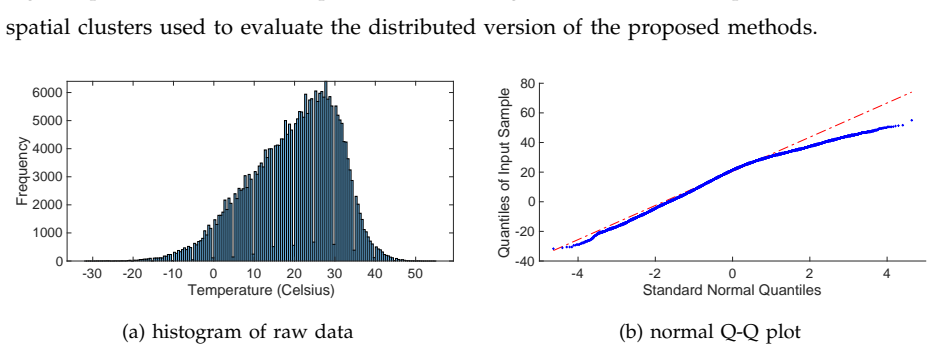
- domain assumption GP hyperparameters estimated from 20 days of temperature data are valid for the test days used in the experiment.
Cite this review
Pith. "Pith review of Bayesian Spatial Field Reconstruction with Unknown Distortions in Sensor Networks." pith.science (2026). https://pith.science/paper/ZFUXK35S
@misc{pith2026190805835,
  author       = {Pith},
  title        = {Pith review of: Bayesian Spatial Field Reconstruction with Unknown Distortions in Sensor Networks},
  year         = {2026},
  howpublished = {\url{https://pith.science/paper/ZFUXK35S}},
  note         = {Machine review of arXiv:1908.05835}
}
read the original abstract
Spatial regression of random fields based on potentially biased sensing information is proposed in this paper. One major concern in such applications is that since it is not known a-priori what the accuracy of the collected data from each sensor is, the performance can be negatively affected if the collected information is not fused appropriately. For example, the data collector may measure the phenomenon inappropriately, or alternatively, the sensors could be out of calibration, thus introducing random gain and bias to the measurement process. Such readings would be systematically distorted, leading to incorrect estimation of the spatial field. To combat this detrimental effect, we develop a robust version of the spatial field model based on a mixture of Gaussian process experts. We then develop two different approaches for Bayesian spatial field reconstruction: the first algorithm is the Spatial Best Linear Unbiased Estimator (S-BLUE), in which one considers the quadratic loss function and restricts the estimator to the linear family of transformations; the second algorithm is based on empirical Bayes, which utilises a two-stage estimation procedure to produce accurate predictive inference in the presence of "misbehaving" sensors. In addition, we develop the distributed version of these two approaches to drastically improve the computational efficiency in large-scale settings. We present extensive simulation results using both synthetic datasets and semi-synthetic datasets with real temperature measurements and simulated distortions to draw useful conclusions regarding the performance of each of the algorithms.
Figures


Figures from the paper (11 more)





Reference graph
Works this paper leans on
-
[1]
Estima tion of Spatially Correlated Random Fields in Heterogeneous Wireless Sensor Networks,
I. Nevat, G. W. Peters, F. Septier, and T. Matsui, “Estima tion of Spatially Correlated Random Fields in Heterogeneous Wireless Sensor Networks,” IEEE T ransactions on Signal Processing , vol. 63, no. 10, pp. 2597– 2609, 2015. 2, 3, 4
work page 2015
-
[2]
Optimal multi-type s ensor placements in gaussian spatial fields for environmental monitoring,
C. Sun, Y . Yu, V . O. Li, and J. C. Lam, “Optimal multi-type s ensor placements in gaussian spatial fields for environmental monitoring,” in 2018 IEEE International Smart Cities Conference (ISC2) . IEEE, 2018, pp. 1–8. 2, 3, 4 39
work page 2018
-
[3]
Short-ter m solar power forecasting based on weighted gaussian process regression,
H. Sheng, J. Xiao, Y . Cheng, Q. Ni, and S. Wang, “Short-ter m solar power forecasting based on weighted gaussian process regression,” IEEE T ransactions on Industrial Electronics , vol. 65, no. 1, pp. 300–308, 2018. 2, 4
work page 2018
-
[4]
K. Sohraby , D. Minoli, and T. Znati, Wireless sensor networks: technology, protocols, and appl ications. John Wiley & Sons, 2007. 2
work page 2007
-
[5]
De centralized hypothesis testing in wireless sensor networks in the presence of misbehaving nodes,
E. Soltanmohammadi, M. Orooji, and M. Naraghi-Pour, “De centralized hypothesis testing in wireless sensor networks in the presence of misbehaving nodes,” IEEE T ransactions on Information Forensics and Security , vol. 8, no. 1, pp. 205–215, 2013. 2
work page 2013
-
[6]
Calibration of mul ti-target tracking algorithms using non-cooperative targets,
B. Ristic, D. E. Clark, and N. Gordon, “Calibration of mul ti-target tracking algorithms using non-cooperative targets,” IEEE Journal of Selected T opics in Signal Processing , vol. 7, no. 3, pp. 390–398, 2013. 2
work page 2013
-
[7]
Draft roadmap for next generation air monit oring,
T. Watkins, “Draft roadmap for next generation air monit oring,” Environmental Protection Agency , 2013. 2
work page 2013
-
[8]
Model-based ren dezvous calibration of mobile sensor networks for monitoring air quality ,
A. Arfire, A. Marjovi, and A. Martinoli, “Model-based ren dezvous calibration of mobile sensor networks for monitoring air quality ,” in 2015 IEEE SENSORS . IEEE, 2015, pp. 1–4. 2
work page 2015
Show all 35 references
-
[9]
Random access sen sor networks: Field reconstruction from incomplete data,
F. Fazel, M. Fazel, and M. Stojanovic, “Random access sen sor networks: Field reconstruction from incomplete data,” in 2012 Information Theory and Applications Workshop . IEEE, 2012, pp. 300–305. 2
2012
-
[10]
Quality of information in mobile crowdsensing: Survey and research challenges,
F. Restuccia, N. Ghosh, S. Bhattacharjee, S. K. Das, and T. Melodia, “Quality of information in mobile crowdsensing: Survey and research challenges,” ACM T ransactions on Sensor Networks (TOSN) , vol. 13, no. 4, p. 34, 2017. 2
2017
-
[11]
Using multi-parameters for calibr ation of low-cost sensors in urban environment,
X. Fang and I. Bate, “Using multi-parameters for calibr ation of low-cost sensors in urban environment,” in Proceedings of the 2017 International Conference on Embedd ed Wireless Systems and Networks . Junction Publishing, 2017, pp. 1–11. 2
2017
-
[12]
Possible artifacts of data biases in the recen t global surface warming hiatus,
T. R. Karl, A. Arguez, B. Huang, J. H. Lawrimore, J. R. McM ahon, M. J. Menne, T. C. Peterson, R. S. V ose, and H.-M. Zhang, “Possible artifacts of data biases in the recen t global surface warming hiatus,” Science, vol. 348, no. 6242, pp. 1469–1472, 2015. 2
2015
-
[13]
Convex o ptimization approaches for blind sensor calibration using sparsity ,
C ¸ . Bilen, G. Puy , R. Gribonval, and L. Daudet, “Convex o ptimization approaches for blind sensor calibration using sparsity ,” IEEE T ransactions on Signal Processing , vol. 62, no. 18, pp. 4847–4856, 2014. 2
2014
-
[14]
On re ndezvous in mobile sensing networks,
O. Saukh, D. Hasenfratz, C. Walser, and L. Thiele, “On re ndezvous in mobile sensing networks,” in Real-World Wireless Sensor Networks . Springer, 2014, pp. 29–42. 2, 6
2014
-
[15]
Info rmed nonnegative matrix factorization methods for mobile sensor network calibration,
C. Dorffer, M. Puigt, G. Delmaire, and G. Roussel, “Info rmed nonnegative matrix factorization methods for mobile sensor network calibration,” IEEE T ransactions on Signal and Information Processing ove r Networks , vol. 4, no. 4, pp. 667–682, 2018. 2, 6
2018
-
[16]
Sensor calibration fo r off-the-grid spectral estimation,
Y . C. Eldar, W. Liao, and S. Tang, “Sensor calibration fo r off-the-grid spectral estimation,” Applied and Computational Harmonic Analysis , 2018. 2
2018
-
[17]
A non-convex approach to joi nt sensor calibration and spectrum estimation,
M. Cho, W. Liao, and Y . Chi, “A non-convex approach to joi nt sensor calibration and spectrum estimation,” in 2018 IEEE Statistical Signal Processing Workshop (SSP) . IEEE, 2018, pp. 398–402. 2
2018
-
[18]
A secure opti mum distributed detection scheme in under-attack wireless sensor networks,
E. Nurellari, D. McLernon, and M. Ghogho, “A secure opti mum distributed detection scheme in under-attack wireless sensor networks,” IEEE T ransactions on Signal and Information Processing ove r Networks , vol. 4, no. 2, pp. 325–337, 2018. 2
2018
-
[19]
Collaborative spectrum sensing in the presence of byzantine attacks in cognitive radio networks,
A. S. Rawat, P . Anand, H. Chen, and P . K. Varshney , “Collaborative spectrum sensing in the presence of byzantine attacks in cognitive radio networks,” IEEE T ransactions on Signal Processing , vol. 59, no. 2, pp. 774–786, 2010. 3
2010
-
[20]
Distributed ev ent detection under byzantine attack in wireless sensor 40 networks,
P . Zhang, J. Y . Koh, S. Lin, and I. Nevat, “Distributed ev ent detection under byzantine attack in wireless sensor 40 networks,” in 2014 IEEE Ninth International Conference on Intelligent Se nsors, Sensor Networks and Information Processing (ISSNIP) . IEEE, 2014, pp. 1–6. 3
2014
-
[21]
Crowdsourcing urban survei llance: The development of homeland security markets for environmental sensor networks,
T. Monahan and J. T. Mokos, “Crowdsourcing urban survei llance: The development of homeland security markets for environmental sensor networks,” Geoforum, vol. 49, pp. 279–288, 2013. 3
2013
-
[22]
Crowd-based learning of spatial fields for the internet of things: From harvesting of data to inference,
E. Arias-de Reyna, P . Closas, D. Dardari, and P . M. Djuri c, “Crowd-based learning of spatial fields for the internet of things: From harvesting of data to inference,” IEEE Signal Processing Magazine , vol. 35, no. 5, pp. 130–139, 2018. 3
2018
-
[23]
Spatial field reconstruction and sensor selection in heterogeneous sensor networks with stochastic energy ha rvesting,
P . Zhang, I. Nevat, G. W. Peters, F. Septier, and M. A. Osb orne, “Spatial field reconstruction and sensor selection in heterogeneous sensor networks with stochastic energy ha rvesting,” IEEE T ransactions on Signal Processing , vol. 66, no. 9, pp. 2245–2257, 2018. 3
2018
-
[24]
How to Utilize Sen sor Network Data to Efficiently Perform Model Calibration and Spatial Field Reconstruction,
G. W. Peters, I. Nevat, and T. Matsui, “How to Utilize Sen sor Network Data to Efficiently Perform Model Calibration and Spatial Field Reconstruction,” in Modern Methodology and Applications in Spatial-T emporal Modeling. Springer, 2015, pp. 25–62. 3
2015
-
[25]
Random Field Reconstruction With Quantization in Wireless Sensor Networks,
I. Nevat, G. W. Peters, and I. B. Collings, “Random Field Reconstruction With Quantization in Wireless Sensor Networks,” IEEE T ransactions on Signal Processing , vol. 61, pp. 6020–6033, 2013. 3, 4
2013
-
[26]
Sampling and reconst ruction of spatial fields using mobile sensors,
J. Unnikrishnan and M. V etterli, “Sampling and reconst ruction of spatial fields using mobile sensors,” IEEE T ransactions on Signal Processing , vol. 61, no. 9, pp. 2328–2340, 2013. 3
2013
-
[27]
Estimating spatial averages of envi ronmental parameters based on mobile crowdsensing,
I. Koukoutsidis, “Estimating spatial averages of envi ronmental parameters based on mobile crowdsensing,” ACM T ransactions on Sensor Networks (TOSN) , vol. 14, no. 1, pp. 1–26, 2017. 3
2017
-
[28]
A trust-base d mixture of gaussian processes model for reliable regression in participatory sensing
Q. Xiang, J. Zhang, I. Nevat, and P . Zhang, “A trust-base d mixture of gaussian processes model for reliable regression in participatory sensing.” in IJCAI, 2017, pp. 3866–3872. 3, 4
2017
-
[29]
Location-aw are cooperative spectrum sensing via Gaussian Processes,
I. Nevat, G. W. Peters, and I. B. Collings, “Location-aw are cooperative spectrum sensing via Gaussian Processes,” in Communications Theory Workshop (AusCTW), 2012 Australian . IEEE, 2012, pp. 19–24. 4
2012
-
[30]
C. E. Rasmussen and C. K. I. Williams, Gaussian Processes for Machine Learning (Adaptive Computa tion and Machine Learning). The MIT Press, 2005. 5, 11, 32
2005
-
[31]
Calibree: A self-calibration system for mobile sensor networks,
E. Miluzzo, N. D. Lane, A. T. Campbell, and R. Olfati-Sab er, “Calibree: A self-calibration system for mobile sensor networks,” in International Conference on Distributed Computing in Sens or Systems . Springer, 2008, pp. 314–331. 6
2008
-
[32]
The cross-entropy method for combinat orial and continuous optimization,
R. Rubinstein, “The cross-entropy method for combinat orial and continuous optimization,” Methodology and computing in applied probability , vol. 1, no. 2, pp. 127–190, 1999. 14
1999
-
[33]
A gentle tutorial of the em algorithm and its application t o parameter estimation for gaussian mixture and hidden markov models,
J. A. Bilmes et al., “A gentle tutorial of the em algorithm and its application t o parameter estimation for gaussian mixture and hidden markov models,” 1998. 16
1998
-
[34]
On the statistical analysis of dirty picture s,
J. Besag, “On the statistical analysis of dirty picture s,” Journal of the Royal Statistical Society: Series B (Methodo log- ical), vol. 48, no. 3, pp. 259–279, 1986. 17
1986
-
[35]
Friedman, T
J. Friedman, T. Hastie, and R. Tibshirani, The elements of statistical learning . Springer series in statistics New York, 2001, vol. 1, no. 10. 33 41 APPENDIX A PROOF OF THEOREMS A. Proof of Theorem 1 Proof. For n = 1, . . . , N, the log model likelihood given f := (f (xn))n=1...
2001
Reviewed August 14, 2026 · model on record in the stance chip above.
Discussion (0). Continue with ORCID to comment.