REVIEW 2 major objections 4 minor 23 references
Non-asymptotic Closed-Loop System Identification using Autoregressive Processes and Hankel Model Reduction
T0 review · 2 major / 4 minor · reviewed 2026-08-14 · deepseek-v4-flash
Pith's one-line read This paper proves a finite-sample upper bound on the prediction error of a closed-loop identification algorithm that fits a long VARX model and then applies Hankel model reduction.
desk verdict First finite-sample bound for closed-loop VARX + balanced reduction, but the proof has a real eigenvalue-direction gap that needs fixing before the rate is established. read the letter →
The pith
A machine-rendered reading of the paper's core claim, the machinery that carries it, and where it could break.
The reading
What carries the argument
The load-bearing object is the REDAR estimator, $\hat y_t = H_R(q)z_t$, obtained from two steps: a ridge-regularized least-squares fit of $y_t$ on $p$ lags of the input/output vector (the VARX step), and balanced model reduction of the fitted transfer matrix with a guaranteed H∞ error at most $\varphi$. The proof decomposes the prediction error into four parts — the optimal noise floor $\|e\|_P^2$, the tail of the steady-state Kalman filter operator $H_\star$, the model-reduction error, and the finite-data least-squares error — and bounds each separately. The finite-data term is controlled by Gaussian concentration on the closed-loop regressor vector, namely a quadratic-form tail bound from the Gaussian moment generating function and a union bound over the entries of the empirical covariance and cross-covariance matrices.
What would settle it
Run REDAR on a stable closed-loop LTI system with identical noise covariances but non-Gaussian heavy-tailed noises (e.g., Student-t or Laplace), and check on fresh data whether the mean squared prediction error decays like $O(1/\sqrt{T})$ and stays below the claimed bound; a violation falsifies the central claim. Equivalent check: compare the empirical tail probabilities of the entries of $\Delta Q$ and $\Delta N$ under such noises with the exponential bound of Lemma 4.
Extended reading notes
Core claim
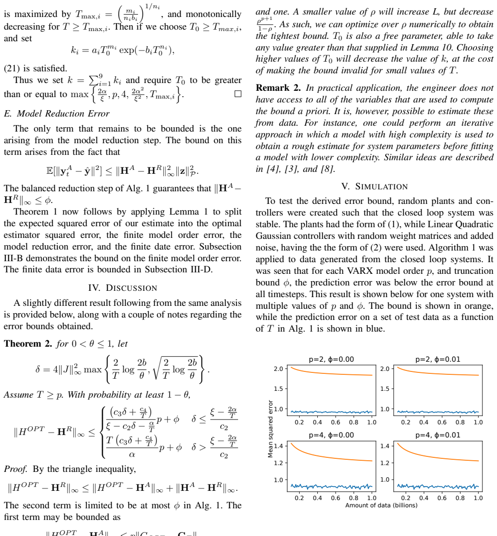
The paper's central claim is Theorem 1. Suppose the steady-state Kalman filter $H_\star(z)$ is bounded by $L$ on or outside a circle of radius $\rho<1$. Then for every $T\ge T_0$ the REDAR predictor $\hat y_t$ satisfies $\mathbb{E}[\|y_t-\hat y_t\|^2] \le \|e\|_P^2 + \frac{L\rho^{p+1}}{1-\rho}\|z\|_P^2 + 2\varphi\|z\|_P^2 + \frac{2k}{\sqrt{T}}\|z\|_P^2$, where $\|e\|_P^2$ is the optimal one-step prediction error of the true model, $z$ stacks the measured input and output, and $k$ and $T_0$ depend on the dimensions, the regularization, the closed-loop H∞ norm, and the minimum noise eigenvalue. The first extra term is the bias from truncating the optimal filter to $p$ past lags, and it decays exponentially in $p$; the second term is the balanced-reduction tolerance; the third is the finite-data estimation error, decaying as $O(1/\sqrt{T})$. The same analysis also gives a high-probability bound on the H∞ distance between the identified predictor and the finite-horizon Kalman filter.
Load-bearing premise
The argument's finite-sample probability bounds assume the process noise and the excitation noise are exactly Gaussian, so the regressor vector is Gaussian; if the noises are not Gaussian, the exponential concentration and the O(1/√T) term are not established by this paper.
Editorial extensions
If this is right
- For any chosen accuracy, an engineer can solve for a sufficient data length T, together with p and φ, from the closed-form bound, giving a sample-complexity certificate for closed-loop identification.
- Because the model-order bias term decays exponentially in p, increasing the VARX order is a cheap way to shrink that term, and the 1/√T finite-data term dominates for large T.
- The balanced-reduction tolerance φ enters linearly, so there is a quantitative trade-off between model simplification and prediction accuracy on unseen closed-loop data.
- The high-probability H∞ bound on the error to the finite-horizon Kalman filter provides a quantified model uncertainty that could support robust control synthesis from finite closed-loop data.
Reading between the lines
- The O(1/√T) rate matches known open-loop non-asymptotic identification rates, suggesting that feedback by itself may not worsen the sample complexity; instead, the closed-loop effect appears in constants such as the closed-loop H∞ norm rather than in the rate.
- The proof structure suggests the same four-term decomposition would work for other reduction schemes, such as Hankel-norm approximation or truncation under a different error metric, whenever an analogous operator error bound is available.
- A natural testable extension is to replace the Gaussian concentration argument with sub-Gaussian or martingale concentration; this would reveal whether the Gaussian assumption is a proof artifact or a real barrier.
- Because the paper's own simulation shows the bound is loose, the practical constants could likely be improved by tightening the intermediate union-bound and norm-estimation steps without changing the algorithm.
Signed reviews
Editorial analysis
A structured set of objections, weighed in public.
Referee Report
Summary. The paper analyzes REDAR, a two-step algorithm that fits a VARX model to closed-loop data and then applies balanced model reduction to obtain a state-space predictor. The main result (Theorem 1) is a non-asymptotic upper bound on the expected squared prediction error, decomposed into the optimal one-step prediction error, a model-order bias term, a model-reduction term, and a finite-data term of order O(1/√T). The proof proceeds through an error decomposition (Lemma 1), a bound on the Kalman filter tail (Lemma 2), concentration inequalities for Gaussian quadratic forms (Lemmas 4-6), and a delta-epsilon argument for the finite-data error (Lemmas 7-10). A second result (Theorem 2) gives a high-probability H∞ bound between the estimated model and the finite-horizon Kalman filter. The paper is self-contained and presents explicit rates, including exponential decay in the autoregressive order p and a 1/√T finite-data term.
Significance. If the bounds are valid, the paper fills a real gap: non-asymptotic guarantees for closed-loop identification are scarce. The algorithm is simple and practically motivated, and the analysis is self-contained, with no fitted constants or circular reasoning. The proof structure is clear, with standard concentration machinery and a clean decomposition of the prediction error into noise, model order, model reduction, and finite-data terms. The paper also provides a high-probability H∞ model-error bound that can be useful for robust control. The main limitation is that the finite-sample bounds require Gaussian noise; for non-Gaussian noise the exponential concentration inequalities are not established.
major comments (2)
- [Theorem 1, model-order term] The proof uses ξ = λmin(Γ) as a lower bound for λmin(Q) when bounding ||Q^{-1}|| by 1/ξ, but the stated inequality ξ ≥ λmin(Q) gives the opposite direction. Since ξ ≥ λmin(Q), we have 1/ξ ≤ ||Q^{-1}||, so the claimed upper bounds in Lemmas 7 and 8 are not valid. A concrete counterexample is the AR(1) system y_t = a y_{t-1} + b u_{t-1} + e_t with u_t = v_t and e_t, v_t iid N(0,1), p=2. The y-y block of Q is (1/(1−a^2))[[1,a],[a,1]] with λmin = 1/(1+|a|), which for a=0.9 equals 0.526, while Γ=I_2 gives ξ=1. Thus Lemma 8's bound 1/(ξ−c2δ−α/T) can be smaller than the true norm ||(Q+ΔQ+α/T I)^{-1}||. Consequently the finite-data error bound in Lemma 10 and the k/√T term in Theorem 1 are not established as written. This is repairable by replacing ξ with λmin(Q) throughout the proof, but the constants in Theorem 1 and Lemma 10 would then depend on λmin(Q) rather than λmin(Γ), so the theorem statement must be revised.
- [Theorem 1, model-order term] The statement of Theorem 1 is inconsistent with the proof in Section III-B. Lemma 2 gives ||H_Tail||∞ ≤ Lρ^{p+1}/(1−ρ), and the bound on E[||y*_{t|−∞:t} − y_head_t||^2] is ||H_Tail||^2∞ ||z||^2_P. The theorem, however, is printed with a term Lρ^{p+1}/(1−ρ) ||z||_P, missing the squares on both the H∞ bound and the signal power. Please correct the theorem statement to match the proof.
minor comments (4)
- [Section III-C, Lemma 4] The eigenvalues of SR are indexed by i=1,...,T+p, but SR is a (T+p)n_z × (T+p)n_z matrix, so there are (T+p)n_z eigenvalues. The subsequent bound uses 2T for the number of eigenvalues; it should be 2Tn_z. This introduces a missing factor of n_z in the concentration constants, which does not change the exponential rate but should be corrected for dimensional consistency.
- [Section III-C, Lemma 5] There is a typo in the statement: the quadratic form should be (z_{t−k})_i (z_{t−ℓ})_j, not (z_{t−k})_i (z_{t−ℓ})_i, since the proof uses e_i e_j^T. Please fix the index.
- [Section II-B and Remark 1] The Gaussian noise assumption is stated in Section II-B, but the discussion would benefit from explicitly noting that the finite-sample concentration bounds are not established for non-Gaussian noise, as this limits their applicability to general industrial data.
- [Theorem 2 and Lemma 6] The probability bound in Theorem 2 uses δ with factor 4||J||^2∞, while Lemma 6 has a factor of 8||J||^2∞ in the linear term after the union bound. Checking the constants would improve the presentation; as printed, the δ expressions appear slightly inconsistent between the lemma and the theorem.
Circularity Check
No circularity: the REDAR generalization bound is a self-contained finite-sample analysis with no fitted parameter renamed as a prediction and no load-bearing self-citation.
full rationale
The paper's central claim, Theorem 1, is an upper bound on the expected prediction error of the REDAR algorithm. The derivation is a self-contained analysis against an assumed closed-loop linear-Gaussian model. The quantities appearing in the bound are not fitted to data: p, alpha, and phi are user-chosen algorithm and approximation parameters; rho and L are assumptions on the true Kalman filter operator; and k and T0 are existential constants produced by the proof rather than estimated values. The finite-sample proof derives concentration inequalities (Lemmas 4-6) from the Gaussian white noise assumption instead of importing them from fitted data, and the finite-data error is analyzed through a deterministic perturbation argument on the least-squares solution rather than by calibrating any constant to match the data. The paper does not rely on self-citations: the reference list contains no works by Lee or Lamperski. External citations, such as the classical balanced model reduction reference and Goldenshluger's autoregressive bounds, are either standard results or are re-proved or modified with proofs included in the paper (e.g., Lemma 2). The method of fitting a VARX model and reducing it is not claimed as a new predictive result but as an analyzed algorithm, so no known empirical pattern is being renamed. The skeptical concern that Lemma 8's inequality involving lambda_min(Gamma) and lambda_min(Q) may be invalid is a possible proof correctness issue, not a circularity issue; an incorrect lemma can invalidate the written proof without making the derivation circular. Overall, no step of the claimed derivation reduces by construction to its own inputs, and no prediction is statistically forced by a fit.
Assumptions & free parameters
assumptions (7)
- domain assumption The true system is an LTI system in innovation form (1) with Gaussian white noise e_t.
- domain assumption The input u_t is generated by the linear feedback controller (2) with Gaussian white excitation v_t independent of e_t.
- domain assumption The closed-loop system is stable, and the joint noise covariance Γ is positive definite.
- domain assumption There exist L > 0 and ρ < 1 such that the Kalman filter transfer function satisfies ||H⋆(z)|| ≤ L for all |z| ≥ ρ.
- domain assumption The closed-loop signal z_t is a Gaussian process, so the stacked vector Z is zero-mean Gaussian with covariance R.
- standard math Balanced model reduction can achieve any H-infinity error tolerance φ, for example by taking the unreduced model when φ is small.
- standard math Standard results: Plancherel theorem, matrix inversion lemma, and Gaussian tail bounds.
Cite this review
Pith. "Pith review of Non-asymptotic Closed-Loop System Identification using Autoregressive Processes and Hankel Model Reduction." pith.science (2026). https://pith.science/paper/ZH35PHVF
@misc{pith2026190902192,
  author       = {Pith},
  title        = {Pith review of: Non-asymptotic Closed-Loop System Identification using Autoregressive Processes and Hankel Model Reduction},
  year         = {2026},
  howpublished = {\url{https://pith.science/paper/ZH35PHVF}},
  note         = {Machine review of arXiv:1909.02192}
}
read the original abstract
One of the primary challenges of system identification is determining how much data is necessary to adequately fit a model. Non-asymptotic characterizations of the performance of system identification methods provide this knowledge. Such characterizations are available for several algorithms performing open-loop identification. Often times, however, data is collected in closed-loop. Application of open-loop identification methods to closed-loop data can result in biased estimates. One method used by subspace identification techniques to eliminate these biases involves first fitting a long-horizon autoregressive model, then performing model reduction. The asymptotic behavior of such algorithms is well characterized, but the non-asymptotic behavior is not. This work provides a non-asymptotic characterization of one particular variant of these algorithms. More specifically, we provide non-asymptotic upper bounds on the generalization error of the produced model, as well as high probability bounds on the difference between the produced model and the finite horizon Kalman Filter.
Figures

Reference graph
Works this paper leans on
-
[1]
Ljung, System identification: theory for the user , 2nd ed
L. Ljung, System identification: theory for the user , 2nd ed. Prentice- hall, 1999
work page 1999
- [2]
-
[3]
Nonparametric estimation of transfer functions: rates of convergence and adaptation,
A. Goldenshluger, “Nonparametric estimation of transfer functions: rates of convergence and adaptation,” IEEE Transactions on Informa- tion Theory, vol. 44, no. 2, pp. 644–658, March 1998
work page 1998
-
[4]
Nonasymptotic bounds for autore- gressive time series modeling,
A. Goldenshluger, A. Zeevi et al., “Nonasymptotic bounds for autore- gressive time series modeling,” The Annals of Statistics, vol. 29, no. 2, pp. 417–444, 2001
work page 2001
-
[5]
Non-Asymptotic Analysis of Robust Control from Coarse-Grained Identification
S. Tu, R. Boczar, A. Packard, and B. Recht, “Non-asymptotic analysis of robust control from coarse-grained identification,” arXiv preprint arXiv:1707.04791, 2017
work page Pith review arXiv 2017
-
[6]
Learning Without Mixing: Towards A Sharp Analysis of Linear System Identification
M. Simchowitz, H. Mania, S. Tu, M. I. Jordan, and B. Recht, “Learning without mixing: Towards a sharp analysis of linear system identification,” arXiv preprint arXiv:1802.08334 , 2018
work page Pith review arXiv 2018
-
[7]
Non-asymptotic identification of lti systems from a single trajectory,
S. Oymak and N. Ozay, “Non-asymptotic identification of lti systems from a single trajectory,” arXiv preprint arXiv:1806.05722 , 2018
arXiv 2018
-
[8]
Finite-Time System Identification for Partially Observed LTI Systems of Unknown Order,
T. Sarkar, A. Rakhlin, and M. A. Dahleh, “Finite-Time System Identification for Partially Observed LTI Systems of Unknown Order,” arXiv e-prints, p. arXiv:1902.01848, Feb 2019
arXiv 1902
Show all 23 references
-
[9]
Learning linear dynamical systems via spectral filtering,
E. Hazan, K. Singh, and C. Zhang, “Learning linear dynamical systems via spectral filtering,” in Advances in Neural Information Processing Systems, 2017, pp. 6702–6712
2017
-
[10]
Spectral filtering for general linear dynamical systems,
E. Hazan, H. Lee, K. Singh, C. Zhang, and Y . Zhang, “Spectral filtering for general linear dynamical systems,” in Advances in Neural Information Processing Systems , 2018, pp. 4634–4643
2018
-
[11]
Introduction to online convex optimization,
E. Hazan et al. , “Introduction to online convex optimization,” Foun- dations and Trends R© in Optimization , vol. 2, no. 3-4, pp. 157–325, 2016
2016
-
[12]
Cesa-Bianchi and G
N. Cesa-Bianchi and G. Lugosi, Prediction, learning, and games . Cambridge university press, 2006
2006
-
[13]
Identification for control: From the early achievements to the revival of experiment design,
M. Gevers, “Identification for control: From the early achievements to the revival of experiment design,” European Journal of Control , vol. 11, pp. 12– 12, 01 2006
2006
-
[14]
On the Sample Complexity of the Linear Quadratic Regulator,
S. Dean, H. Mania, N. Matni, B. Recht, and S. Tu, “On the Sample Complexity of the Linear Quadratic Regulator,” arXiv e-prints , p. arXiv:1710.01688, Oct 2017
2017 arXiv
-
[15]
Closed-loop identification revisited,
U. Forssell and L. Ljung, “Closed-loop identification revisited,” Auto- matica, vol. 35, no. 7, pp. 1215 – 1241, 1999
1999
-
[16]
Subspace identification from closed loop data,
L. Ljung and T. McKelvey, “Subspace identification from closed loop data,” Signal Processing, vol. 52, no. 2, pp. 209 – 215, 1996, subspace Methods, Part II: System Identification
1996
-
[17]
Subspace identification and arx modeling,
M. Jansson, “Subspace identification and arx modeling,” IFAC Pro- ceedings Volumes, vol. 36, no. 16, pp. 1585 – 1590, 2003, 13th IFAC Symposium on System Identification (SYSID 2003), Rotterdam, The Netherlands, 27-29 August, 2003
2003
-
[18]
The role of vector autoregressive modeling in predictor- based subspace identification,
A. Chiuso, “The role of vector autoregressive modeling in predictor- based subspace identification,” Automatica, vol. 43, no. 6, pp. 1034– 1048, 2007
2007
-
[19]
An overview of subspace identification,
S. J. Qin, “An overview of subspace identification,” Computers and Chemical Engineering, vol. 30, no. 10, pp. 1502 – 1513, 2006, papers form Chemical Process Control VII
2006
-
[20]
Closed-loop subspace identification methods: an overview,
G. van der Veen, J.-W. van Wingerden, M. Bergamasco, M. Lovera, and M. Verhaegen, “Closed-loop subspace identification methods: an overview,” IET Control Theory & Applications , vol. 7, no. 10, pp. 1339–1358, 2013
2013
-
[21]
The relation of the cca subspace method to a balanced reduction of an autoregressive model,
A. Dahlen and W. Scherrer, “The relation of the cca subspace method to a balanced reduction of an autoregressive model,” Journal of Econometrics, vol. 118, no. 1-2, pp. 293–312, 2004
2004
-
[22]
K. Zhou, J. C. Doyle, K. Glover et al. , Robust and optimal control . Prentice hall New Jersey, 1996, vol. 40
1996
-
[23]
M. J. Wainwright, High-dimensional statistics: A non-asymptotic view- point. Cambridge University Press, 2019, vol. 48
2019
Reviewed August 14, 2026 · model on record in the stance chip above.
Discussion (0). Continue with ORCID to comment.