Pith. sign in

REVIEW 1 major objections 8 minor 4 references

COST INTERACT Whitepaper on Signal Processing for Communications, Localization, and Intergrated Sensing and Communication

T0 review · 1 major / 8 minor · reviewed 2026-08-11 · deepseek-v4-flash

Pith's one-line read A Bussgang decomposition applies to any signal-noise distribution.

desk verdict A competent, broad 6G signal-processing survey from a COST working group; the only new math is a Bussgang note that is correct but oversold. read the letter →

arxiv 2412.08679 v1 pith:ZOFYYTDK submitted 2024-12-11 eess.SP

classification eess.SP
keywords 6GphysicallayerintegratedsensingandcommunicationlocalizationBussgangdecompositionwaveformdesignmassiveMIMOsecurity
verification ladder T0 review T1 audit T2 compute T3 formal

The pith

A machine-rendered reading of the paper's core claim, the machinery that carries it, and where it could break.

The reading

This whitepaper argues that meeting 6G targets (1 Tbps data rates, 1 ms latency, 1000 km/h speeds, and integrated sensing) requires rethinking the physical layer. Its most concrete technical claim is that the Bussgang decomposition works for any signal and noise distribution, not just Gaussian. The paper derives that an output of a memoryless nonlinearity can be written as a scaled input plus uncorrelated distortion, with coefficients based on conditional moments, and it gives a signal-to-distortion-plus-noise ratio formula valid without Gaussianity. It also surveys and proposes work on waveforms, coding, massive MIMO, massive access, fronthaul compression, security, localization, and ISAC. A sympathetic reader should care because if the Bussgang generalization holds, nonlinear amplifiers can be modeled for non-Gaussian and non-OFDM waveforms that 6G may use.

What carries the argument

The carrying object is the Bussgang decomposition: for a memoryless nonlinearity $y = f(x)$, the output is split as $y = \alpha_x x + \delta_x$, where $\delta_x$ is uncorrelated with $x$ and $\alpha_x = \mathbb{E}[yx]/\mathbb{E}[x^2]$. The generalized version uses conditional moments $\mu_y(s) = \mathbb{E}[y|s]$ and $\mu_{y^2}(s) = \mathbb{E}[y^2|s]$, defining $\alpha_s$ and $\gamma_s$ through integrals over the signal distribution $p_s(s)$. This yields the distribution-free relation $\gamma_s = \gamma_x(1 + \sigma_n^2/\sigma_s^2)$ that anchors the SDNR formula.

What would settle it

Feed a memoryless nonlinearity a sum of a Bernoulli-distributed signal and $\alpha$-stable noise with infinite variance, compute $\alpha_s = \mathbb{E}[ys]/\mathbb{E}[s^2]$, and test whether $y - \alpha_s s$ is uncorrelated with $s$; a nonzero correlation, or a divergence in $\gamma_s$, would falsify the claimed general decomposition. Even within finite variance, a simulation where Eq. (19) fails to predict the measured signal-to-distortion-plus-noise ratio would settle the matter.

Watch

Extended reading notes

Core claim

Section 1.5.6 claims that 'a version of the Bussgang decomposition applies in general, regardless of the distribution of signal and noise.' Writing the input to a memoryless nonlinearity as $x = s + n$ with zero-mean, independent, finite-variance signal and noise, the paper defines $\alpha_s = \mathbb{E}[ys]/\mathbb{E}[s^2]$ and shows that $y - \alpha_s s$ is uncorrelated with $s$. It also defines $\gamma_s = \mathbb{E}[y^2]/\mathbb{E}[s^2]$ and shows that $\gamma_s = \gamma_x (1 + \sigma_n^2/\sigma_s^2)$ holds for arbitrary distributions, while the classical simplification $\alpha_s = \alpha_x$ requires Gaussianity. The resulting signal-to-distortion-plus-noise ratio in Eq. (19) is claimed to hold generally, with Eq. (20) as the Gaussian special case. The paper notes that the distortion-plus-noise term is not usually Gaussian even when the input is.

Load-bearing premise

The generalization assumes the wanted signal and noise are independent zero-mean random variables with finite second moments; if the noise is heavy-tailed, correlated with the signal, or has infinite variance, the derived relations for $\alpha_s$ and $\gamma_s$ no longer follow.

Editorial extensions

If this is right

  • Non-Gaussian waveforms such as OTFS, chirp, and ISAC signals can be analyzed with a linear-plus-uncorrelated-distortion model for nonlinear amplifiers.
  • The SDNR formula gives a way to choose transmit power, backoff, and power allocation under arbitrary signal and noise statistics, assisting distortion-aware precoding and energy-efficient designs.
  • In the Gaussian case, results reduce to the classical Bussgang formulas, so existing receiver designs remain valid as a special case.

Reading between the lines

Editorial extensions of the paper, not claims the author makes directly.

  • A direct test would feed a nonlinear amplifier with a non-Gaussian signal plus heavy-tailed interference and check whether $y - \alpha_s s$ remains uncorrelated with $s$; residual correlation would pinpoint where independence or finite-variance premises break.
  • Quantization is itself a memoryless nonlinearity, so the generalized decomposition could be applied to optimize fronthaul quantization intervals without assuming Gaussian signals.
  • If $\alpha_s$ must be computed from actual distributions, data-driven estimates of $\alpha_s$ may become useful for neural-network receivers and ISAC distortion models.
Share X Bluesky LinkedIn Reddit HN

Signed reviews

No signed human review yet.

Editorial analysis

A structured set of objections, weighed in public.

Desk editor's note, referee report, and a circularity audit.

Referee Report

1 major / 8 minor

Summary. This document is a whitepaper from COST Action INTERACT Working Group 2. It surveys signal processing for communications (waveforms, channel coding, massive MIMO, massive access, RF impairments, O-RAN, security, underwater communications), signal processing for localization (AoA, fingerprinting, SLAM, machine learning, RSSI/UWB/LoRa, RIS, testbeds), and integrated sensing and communication (terminology, resource allocation, waveform design, channel measurements, parameter estimation, WiFi/cellular sensing). It reports a large number of the group's contributions, with heavy citation to internal WG2 papers, and contains one self-contained derivation: a generalized Bussgang decomposition for nonlinear systems with noisy inputs in Section 1.5.6.

Significance. As a survey and roadmap, the whitepaper is useful: it consolidates a broad range of 6G physical-layer topics and documents the activity of a large European working group. Its strengths are its breadth, its connection of each topic to concrete WG2 publications, and the explicit enumeration of open problems. The Bussgang derivation in Section 1.5.6 is internally consistent under the standard assumptions of zero-mean, finite-variance, independent signal and noise, and it gives a useful reminder that the SDNR identity itself does not require Gaussianity. However, the manuscript does not contain a single falsifiable central claim or reproducible experiments; most programmatic statements are qualitative, and many quantitative claims are borrowed from cited papers without providing enough detail for independent verification. As a position or survey document it could be valuable, but its technical authority rests on the cited primary literature rather than on the content of this paper.

major comments (1)
  1. [1.5.6] The statement near Eqs. (14)-(20) that "a version of the Bussgang decomposition applies in general, regardless of the distribution of signal and noise" is an overstatement. The derivation of γs = γx(1 + σ_n^2/σ_s^2) and the SDNR formula in Eq. (19) presupposes that s and n are zero-mean, finite-variance, and uncorrelated (in the intended setting, independent), because it uses E[x^2] = σ_s^2 + σ_n^2. If n = s, then σ_n^2 = σ_s^2 but E[x^2] = 4σ_s^2, so γs = 4γx rather than the 2γx that Eq. (19) would give; if n is α-stable with α < 2, σ_n^2 is undefined and the formula is not meaningful. Moreover, for arbitrary distributions the decomposition y = αs s + δs with δs uncorrelated with s is a linear orthogonal projection (linear MMSE), not the Bussgang constant-gain property, and the paper itself concedes that αs depends on the distributions of s and n. Please state the required assumptions explicitly before Eq. (14) and replace the unqualified "regardless of distribution" claim with a qualification such as "for zero-mean, finite-variance, uncorrelated signal and noise; in the general case the decomposition reduces to the linear MMSE/projection property."
minor comments (8)
  1. [Title] The title contains a typo: "Intergrated" should be "Integrated."
  2. [1.5.6] The notation is inconsistent: the text before Eq. (11) refers to the input standard deviation as σ, whereas Eq. (11) uses σx, and the noisy-case definitions of σs and σn do not state the independence or finite-variance assumptions. Please align the notation and place the assumptions with the definitions.
  3. [1.6.2] The density PN in Eq. (23) is not defined; please define it explicitly (presumably the noise PDF) before using it in the mutual-information expression.
  4. [1.8] There are several typos: "see water" should be "sea water," "Baltic See" should be "Baltic Sea," and the citation "[P.521]" does not match the "ITU-R Recommendation P.527-6" mentioned in the same sentence.
  5. [1.4.2] The maximum-likelihood expression in Eq. (2) is garbled; the minimization should be over b ∈ {0,1}^N and the norm should be written explicitly, for example as || y - Σ_{i=1}^N h_i b_i c_i ||^2.
  6. [1.5.2] The phrase "Voltera series" should be "Volterra series."
  7. [1.5.6] The caveat in the last paragraph, that the distortion-plus-noise term is not generally Gaussian even in the Gaussian-input case, limits the usefulness of the SDNR formula for BER analysis; move this caveat immediately after Eq. (19) so that it appears together with the SDNR claim.
  8. [1.6.2] In Figures 9 and 10, the legend labels "mq 3" and "mq 4" are unclear; please use m_q = 3, m_q = 4 or define the notation in the caption.

Circularity Check

0 steps flagged · score 0.0 of 10

No significant circularity: the whitepaper's self-citations are descriptive summaries, and the one novel derivation (generalized Bussgang decomposition) is algebraic and self-contained.

full rationale

The document is a position/whitepaper rather than a research derivation chain. Its self-citations (e.g., BS22, BV22, BS24, Baj23, PR23b) are used to describe past contributions of WG2 members, not as load-bearing premises that force new conclusions. The only substantive new derivation is the noisy-case Bussgang decomposition in Section 1.5.6, Eqs. (14)-(20). That derivation is self-contained: alpha_s is defined as the projection coefficient E[ys]/E[s^2] (Eq. 15), which by construction makes y - alpha_s s uncorrelated with s; gamma_s = gamma_x (1 + sigma_n^2 / sigma_s^2) follows algebraically from E[x^2] = sigma_s^2 + sigma_n^2 under the usual zero-mean and uncorrelated signal/noise assumptions. No fitted parameter is relabeled as a prediction, and no uniqueness theorem from the authors' prior work is invoked to force a choice. The phrase 'regardless of the distribution of signal and noise' overstates the assumptions needed (independence and finite second moments), and the paper itself notes the non-Gaussianity of the distortion-plus-noise term, but these are correctness/qualification concerns, not circularity. The abundant self-citations are descriptive and do not reduce any claimed result to an input of the whitepaper.

Assumptions & free parameters 0 free parameters · 4 assumptions · 0 invented entities

The document is a review, so the ledger mostly records modeling assumptions used in its few concrete derivations and simulations. There are no free parameters or invented entities.

assumptions (4)
  • domain assumption The power amplifier is modeled as a memoryless nonlinear function f(x).
    Section 1.5.6 builds the Bussgang decomposition on this model; real PAs have memory effects, but the memoryless assumption is standard in this analysis.
  • domain assumption Signal s and noise n are independent, zero-mean random variables with finite second moments.
    Used in Equations (14)-(20) to derive alpha_s and gamma_s; independence is required for E[x^2] = sigma_s^2 + sigma_n^2.
  • domain assumption The surveyed literature, including many self-citations, accurately represents the state of the art.
    The whitepaper's value depends on the correctness of its summaries; no independent verification is provided for each cited result.
  • domain assumption Standard stochastic channel models (AWGN, Rayleigh block-faded) are used where simulation results are presented.
    For example, the fronthaul compression analysis in Section 1.6.2 assumes AWGN with QPSK and LDPC codes.

how reviews work

0 comments
Cite this review

Pith. "Pith review of COST INTERACT Whitepaper on Signal Processing for Communications, Localization, and Intergrated Sensing and Communication." pith.science (2026). https://pith.science/paper/ZOFYYTDK

@misc{pith2026241208679,
  author       = {Pith},
  title        = {Pith review of: COST INTERACT Whitepaper on Signal Processing for Communications, Localization, and Intergrated Sensing and Communication},
  year         = {2026},
  howpublished = {\url{https://pith.science/paper/ZOFYYTDK}},
  note         = {Machine review of arXiv:2412.08679}
}
read the original abstract

The upcoming next generation of wireless communication is anticipated to revolutionize the conventional functionalities of the network by adding sensing and localization capabilities, low-power communication, wireless brain computer interactions, massive robotics and autonomous systems connection. Furthermore, the key performance indicators expected for the 6G of mobile communications promise challenging operating conditions, such as user data rates of 1 Tbps, end-to-end latency of less than 1 ms, and vehicle speeds of 1000 km per hour. This evolution needs new techniques, not only to improve communications, but also to provide localization and sensing with an efficient use of the radio resources. The goal of INTERACT Working Group 2 is to design novel physical layer technologies that can meet these KPI, by combining the data information from statistical learning with the theoretical knowledge of the transmitted signal structure. Waveforms and coding, advanced multiple-input multiple-output and all the required signal processing, in sub-6-GHz, millimeter-wave bands and upper-mid-band, are considered while aiming at designing these new communications, positioning and localization techniques. This White Paper summarizes our main approaches and contributions.

Figures

Figures reproduced from arXiv: 2412.08679 by the authors.

Figure 1
Figure 1. 6G waveforms directions and design criteria. [PITH_FULL_IMAGE:figures/full_fig_p009_1.png] view at source ↗
Figure 2
Figure 2. The general concept of GMSK detector. 27 [PITH_FULL_IMAGE:figures/full_fig_p027_2.png] view at source ↗
Figure 3
Figure 3. The DL-based phase corrector structure. The presented model consists of convolutional and feedforward neural networks connected with a flattened layer. The output of the network represents the estimated phase θ rotation in terms of sinθ and cosθ representation. The accuracy of the performed phase correction for exemplary packet and EPA channel outperforms the state-of-the-art methods. 1.5.5 Wideband and ultra-wideba… view at source ↗
Figures from the paper (99 more)
Figure 4
Figure 4. Figure 4: O-RAN Architecture [MH23] The O-RAN architecture, as shown in [PITH_FULL_IMAGE:figures/full_fig_p031_4.png]
Figure 5
Figure 5. Figure 5: RAN Protocol and RRM control into the open-central unit control plane (O-CU-CP), responsible for tasks such as radio resource man￾agement and handover decisions, and the open-central unit user plane (O-CU-UP), which handles user data traffic, including encryption, decr…
Figure 6
Figure 6. Figure 6: 3GPP Specific RAN Disaggregation Options [PITH_FULL_IMAGE:figures/full_fig_p033_6.png]
Figure 7
Figure 7. Figure 7: RAN Disaggregation and Distributed Deployment [PITH_FULL_IMAGE:figures/full_fig_p033_7.png]
Figure 8
Figure 8. Figure 8: CU-DU-RU Disaggregation The second tier of disaggregation is vertical and focuses on separating the control and user planes within the O-CU. This disaggregates the O-CU into: • O-CU-UP: Manages the user-plane part of PDCP and SDAP protocols. • O-CU-CP: Handles the cont…
Figure 9
Figure 9. Figure 9: Finding optimum ∆ (SNR -8dB). 0 0.05 0.1 0.15 0.2 Delta 1.2 1.3 1.4 1.5 1.6 1.7 1.8 1.9 2 2.1 2.2 MI 10 -3 10 -2 10 -1 10 0 BLER mq 4 mq 5 mq 6 mq 4 mq 5 mq 6 [PITH_FULL_IMAGE:figures/full_fig_p037_9.png]
Figure 11
Figure 11. Figure 11: BLER-SNR curves for MCS 0-23 (left to right). Optimum quantized results shown as black [PITH_FULL_IMAGE:figures/full_fig_p038_11.png]
Figure 12
Figure 12. Figure 12: An illustration depicting the CIAA quartet as the foundational pillars of wireless security. [PITH_FULL_IMAGE:figures/full_fig_p039_12.png]
Figure 13
Figure 13. Figure 13: An overview of key requirements for 6G networks. [PITH_FULL_IMAGE:figures/full_fig_p040_13.png]
Figure 14
Figure 14. Figure 14: Schematic representation of the primary functions of wireless threats. [PITH_FULL_IMAGE:figures/full_fig_p041_14.png]
Figure 15
Figure 15. Figure 15: A schematic representation of symmetric cryptography. [PITH_FULL_IMAGE:figures/full_fig_p041_15.png]
Figure 16
Figure 16. Figure 16: A schematic representation of asymmetric cryptography. [PITH_FULL_IMAGE:figures/full_fig_p042_16.png]
Figure 17
Figure 17. Figure 17: Basic illustration for anti-jamming based [PITH_FULL_IMAGE:figures/full_fig_p045_17.png]
Figure 18
Figure 18. Figure 18: Illustration of anti-jamming techniques: (a) spread spectrum, (b) cooperative relay, and [PITH_FULL_IMAGE:figures/full_fig_p046_18.png]
Figure 19
Figure 19. Figure 19: Illustration of existing physical layer authentication techniques: (a) channel-based authen [PITH_FULL_IMAGE:figures/full_fig_p046_19.png]
Figure 20
Figure 20. Figure 20: An illustration of different NTN deployments. [PITH_FULL_IMAGE:figures/full_fig_p047_20.png]
Figure 21
Figure 21. Figure 21: The sound speed profile plot￾ted with Bellhop [bel] tool according to data from Baltic Sea measured in 2019.08.21 given in [BD21] [PITH_FULL_IMAGE:figures/full_fig_p051_21.png]
Figure 23
Figure 23. Figure 23: Fingerprinting method Fingerprinting consists of two distinct phases, as depicted in [PITH_FULL_IMAGE:figures/full_fig_p055_23.png]
Figure 24
Figure 24. Figure 24: Random Forest scheme forward due to their use of decision trees, resulting in computational efficiency. Additionally, Random Forest are robust to data noise, as the averaging of outputs from multiple decision trees helps mitigate the impact of any single inaccurate es…
Figure 25
Figure 25. Figure 25: CDF of the error of different methods with 5G data [PITH_FULL_IMAGE:figures/full_fig_p060_25.png]
Figure 26
Figure 26. Figure 26: Comparison of simulated normalized root mean squared positioning error and uncertainty [PITH_FULL_IMAGE:figures/full_fig_p061_26.png]
Figure 27
Figure 27. Figure 27: Performance comparison of base DNN and wireless transformer (WiT) [ [PITH_FULL_IMAGE:figures/full_fig_p061_27.png]
Figure 28
Figure 28. Figure 28: Performance comparison of base wireless transformer (WiT) and self-supervised wireless [PITH_FULL_IMAGE:figures/full_fig_p062_28.png]
Figure 29
Figure 29. Figure 29: The idea of multipath assisted positioning is to treat every MPC as a [PITH_FULL_IMAGE:figures/full_fig_p062_29.png]
Figure 30
Figure 30. Figure 30: The flow chart of a fingerprinting scheme using Channel-SLAM for collecting fingerprints [PITH_FULL_IMAGE:figures/full_fig_p063_30.png]
Figure 31
Figure 31. Figure 31: A top view of the simulation scenario with one physical transmitter labeled transmitter ( [PITH_FULL_IMAGE:figures/full_fig_p064_31.png]
Figure 32
Figure 32. Figure 32: Results for different numbers of components in the MDN GMM. [PITH_FULL_IMAGE:figures/full_fig_p064_32.png]
Figure 34
Figure 34. Figure 34: root mean square error (RMSE) of compared cooperative localization algorithms. simpler, ideal for weight-sensitive UAV and less complex devices, despite its susceptibility to noise and signal distortion. While RSSI localization is widely adopted for its speed and cost…
Figure 35
Figure 35. Figure 35: Beacon indoor experimental area setup. With respect to complex indoor environments, they could be challenging scenarios due to multipath and NLOS effects that are known to cause errors in ranging and positioning [DCD15]. In these setups, technologies such as WiFi stan…
Figure 36
Figure 36. Figure 36: Dataset was collected at the Indoor Navigation Laboratory of the CTTC [ [PITH_FULL_IMAGE:figures/full_fig_p075_36.png]
Figure 37
Figure 37. Figure 37: Scenarios (left) from [Mor22] with node placements in the map of the lab. The red triangles are the anchor UWB nodes and the black dot is the target UWB node. The table (right) shows the propagation and geometry conditions of each anchor node in the scenarios. Scenari…
Figure 38
Figure 38. Figure 38: RMSE of the target node position with Scenario A2 (left) and A3 zoom (right) [PITH_FULL_IMAGE:figures/full_fig_p076_38.png]
Figure 39
Figure 39. Figure 39: RMSE of the target node position with Scenario A3 (left) and A4 (right). did not diverge. It can be seen that the algorithm iterations reduced the error, but the FG algorithm with WLS (’WLS with FG’) needed more iterations than the iterative WLS (’WLS’ in figure legen…
Figure 40
Figure 40. Figure 40: RMSE of the target node position with Scenario B (left) and C2 (right). 76 [PITH_FULL_IMAGE:figures/full_fig_p076_40.png]
Figure 41
Figure 41. Figure 41: Indoor measurements environments: [left] Hall, [middle] Locker room, and [right] Corridor. [PITH_FULL_IMAGE:figures/full_fig_p079_41.png]
Figure 42
Figure 42. Figure 42: Floor plan of the environment Hall (green and red dots mark the positions of Tx and receiver (Rx)) and localization errors in the environment Hall [SP22]. sensitivity -low bandwidth (BW) and high spreading factor (SF) - and lowest sensitivity - high BW and low SF -. T…
Figure 43
Figure 43. Figure 43: Floor plan of the environment Locker room (green and red dots mark the positions of Tx and Rx) and localization errors in the environment Locker Room [SP22]. 3.0 m 18.9 m A B C D P 3 P 2 P 1 [PITH_FULL_IMAGE:figures/full_fig_p080_43.png]
Figure 44
Figure 44. Figure 44: Floor plan of the environment Corridor (green and red dots mark the positions of Tx and Rx) and localization errors in the environment Corridor [SP22]. 80 [PITH_FULL_IMAGE:figures/full_fig_p080_44.png]
Figure 46
Figure 46. Figure 46: The receiver parameters To configure the USRPs, we use GNU Radio framework with its graphical interface known as GNU Radio Companion. In the receiving mode, the 2 types of blocks are designed: USRP source and file meta sink. USRP source block interfaces with the USRP …
Figure 47
Figure 47. Figure 47: Map of the testing scenario [PITH_FULL_IMAGE:figures/full_fig_p083_47.png]
Figure 48
Figure 48. Figure 48: Localization error through fields [PITH_FULL_IMAGE:figures/full_fig_p084_48.png]
Figure 50
Figure 50. Figure 50: Localization error though fields for after smoothing the detected coordinates [PITH_FULL_IMAGE:figures/full_fig_p084_50.png]
Figure 52
Figure 52. Figure 52: HOP-5G dedicated and aerial 5G positioning testbed [ [PITH_FULL_IMAGE:figures/full_fig_p089_52.png]
Figure 53
Figure 53. Figure 53: Mission scenario on Mt. Etna robots with attached [PITH_FULL_IMAGE:figures/full_fig_p089_53.png]
Figure 54
Figure 54. Figure 54: 3D position and orientation estimation [ [PITH_FULL_IMAGE:figures/full_fig_p090_54.png]
Figure 55
Figure 55. Figure 55: Sensor eggs deployed on the fumarole field of the volcano “La Fossa”, Vulcano, Italy [PITH_FULL_IMAGE:figures/full_fig_p090_55.png]
Figure 56
Figure 56. Figure 56: Sensor eggs deployed in a lava cave on Lanzarote, Spain. [PITH_FULL_IMAGE:figures/full_fig_p091_56.png]
Figure 57
Figure 57. Figure 57: The LOG-a-TEC testbed, with the position of the nodes. [PITH_FULL_IMAGE:figures/full_fig_p091_57.png]
Figure 58
Figure 58. Figure 58: Communication and radio sensing on . localization, the target actively transmits a signal for detection and localization purposes. Typical applications of detection and tracking include surveillance, automotive driving, and robotics [PITH_FULL_IMAGE:figures/full_fig_…
Figure 59
Figure 59. Figure 59: ISAC Applications: detection and tracking, environmental sensing, smart human interac￾tion, and imaging. as illustrated Environmental sensing employs radio signals to determine the condition of the air, including the presence of dust, as well as to predict weather pat…
Figure 60
Figure 60. Figure 60: Integration levels: co-existent, cooperating, and collaborative systems [PITH_FULL_IMAGE:figures/full_fig_p093_60.png]
Figure 61
Figure 61. Figure 61: Underlying systems: Communication-centric, radar-centric, and co-design [PITH_FULL_IMAGE:figures/full_fig_p094_61.png]
Figure 62
Figure 62. Figure 62: Link constellations: Monostatic, bistatic, and mulit-static [PITH_FULL_IMAGE:figures/full_fig_p095_62.png]
Figure 63
Figure 63. Figure 63: (a) An illustration of an ISAC system with TDD communication and ’duplex’ monostatic sensing [AKM23], where the use of auxillary aperture is to assist the JCAS aperture to form ’duplex’ monostatic sensing. For instance, when JCAS aperture forms multiple transmitting b…
Figure 64
Figure 64. Figure 64: An illustration of an ISAC system with fully shared aperture: each antenna is connected to a unit working as both LNA or PA at the back plane of the array, and then to up/down converters that are switch-able. This architecture is with TDD assumption. 96 [PITH_FULL_IM…
Figure 65
Figure 65. Figure 65: Classification of waveform design for ISAC [WQW+23a]. for communications by means of LoRa modulation in long range wide area network (LoRaWAN). We highlight the INTERACT contribution in [SGEX], in which the authors present the waveform structure and receiver processin…
Figure 66
Figure 66. Figure 66: DRL concept with the agent and the environment including the simulation models. DRL is a suitable approach to solve complex problems such as resource allocation. The DRL algorithm solves problems by a decision policy represented by a neural network that has been train…
Figure 67
Figure 67. Figure 67: Radar sensing modes: The search mode in green and the track mode in red. Allocated [PITH_FULL_IMAGE:figures/full_fig_p101_67.png]
Figure 68
Figure 68. Figure 68: Averaged allocated power (left) and Averaged Observation losses by an agent selecting [PITH_FULL_IMAGE:figures/full_fig_p102_68.png]
Figure 69
Figure 69. Figure 69: 5G NR frame structure vs. proposed downlink BM frame structure. non-cooperative targets typically only act as reflectors. Because of their different capabilities, dif￾ferent channel estimate techniques are required, leading to different demands on radio resources and …
Figure 70
Figure 70. Figure 70: Dual-band sensing scenario. (JUST AS A PLACE HOLDER) [PITH_FULL_IMAGE:figures/full_fig_p105_70.png]
Figure 71
Figure 71. Figure 71: Illustration of the concept of guard beam [PITH_FULL_IMAGE:figures/full_fig_p106_71.png]
Figure 72
Figure 72. Figure 72: ISAC-capable Sidelink 5G-V2X Highway Scenario The ISAC-capable sidelink system has distinct performance requirements for radar sensing and communication. The radar sensing requirements include high range and velocity resolution, low de￾tection error, and large sensing…
Figure 73
Figure 73. Figure 73: Workflow of Radar-enabled resource allocation algorithm [PITH_FULL_IMAGE:figures/full_fig_p107_73.png]
Figure 74
Figure 74. Figure 74: Scenario description and antenna setup: (left) A car approaches a “T”- intersection and [PITH_FULL_IMAGE:figures/full_fig_p111_74.png]
Figure 75
Figure 75. Figure 75: Different sensing direction for ve￾hicular ISAC [PITH_FULL_IMAGE:figures/full_fig_p112_75.png]
Figure 77
Figure 77. Figure 77: (Left Up) System configuration of dual-band distributed [PITH_FULL_IMAGE:figures/full_fig_p113_77.png]
Figure 78
Figure 78. Figure 78: Definition of ISAC dual channel model Some new and innovative approaches, such as [NC23], to the dual channel model in ISAC, show great potential for channel sounding. These approaches involve advanced signal processing techniques and sophisticated radar systems to ex…
Figure 79
Figure 79. Figure 79: Flowchart of the channel estimation algorithm and comparison between measured S11, S12 [PITH_FULL_IMAGE:figures/full_fig_p115_79.png]
Figure 80
Figure 80. Figure 80: BiRa measurement range for bistatic radar reflectivity at TU Ilmenau (the Stargate antenna arch is not used in this case). This way we effectively get another dimension besides the four-dimensional (4D) angles. Moreover, the radial distance of Tx and Rx antennas from …
Figure 81
Figure 81. Figure 81: Analyzed scenario for drone detection The analyzed scenario of drone detection in this section is illustrated in [PITH_FULL_IMAGE:figures/full_fig_p118_81.png]
Figure 82
Figure 82. Figure 82: The block diagram of signal processing Parameter Setup System VNA Frequency sweep 2−18 GHz, 1601 steps Static Gantry 10◦ :5◦ :180◦ Dynamic Gantry 90◦ Turn- [PITH_FULL_IMAGE:figures/full_fig_p118_82.png]
Figure 83
Figure 83. Figure 83: Comparison of normalized reflectivity by [PITH_FULL_IMAGE:figures/full_fig_p119_83.png]
Figure 84
Figure 84. Figure 84: Normalized reflectivity of DJI P2 for different bistatic viewing angles (10 [PITH_FULL_IMAGE:figures/full_fig_p119_84.png]
Figure 85
Figure 85. Figure 85: The block diagram of OFDM Micro-Doppler signal processing To achieve this, we follow the signal processing scheme showed in [PITH_FULL_IMAGE:figures/full_fig_p120_85.png]
Figure 86
Figure 86. Figure 86: BiRa micro-Doppler measurement of DJI Phantom II drone, vulnerable road user (VRU) pedestrian model target, and VRU cyclist model target. Pedestrian target: Fig. 86d shows a sample time-Doppler signature of the EPTa produced with Setup 1. The image shows the signal ha…
Figure 87
Figure 87. Figure 87: Scalability between stochastic and deterministic channel modeling components and accuracy [PITH_FULL_IMAGE:figures/full_fig_p123_87.png]
Figure 88
Figure 88. Figure 88: (a) Discretized sphere used for the simulation; Radius 12 [PITH_FULL_IMAGE:figures/full_fig_p123_88.png]
Figure 89
Figure 89. Figure 89: Illustrative case of a human moving their hands outwards (a) Multipaths extracted from the [PITH_FULL_IMAGE:figures/full_fig_p125_89.png]
Figure 90
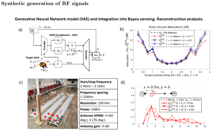
Figure 90. Figure 90: (a) generative neural network (GNN) for reconstruction of RF data - conditional varia￾tional autoencoders (C-VAE) implementation. (b) and (d) Effects of GNN reconstruction on dataset accuracy (comparison between measurement of body-induced attenuations and synthetic R…
Figure 91
Figure 91. Figure 91: Precision/recall metrics for distance estimation. Estimated prior from calibration data, [PITH_FULL_IMAGE:figures/full_fig_p127_91.png]
Figure 92
Figure 92. Figure 92: The architecture of the CNN used in [SSF+]. The network uses mainly convolutional layers, which the number of trainable parameters, enabling multiple dimensions. The predictions contain both the parameters and the model-order of the data. them prime candidates for the…
Figure 93
Figure 93. Figure 93: Delay [PITH_FULL_IMAGE:figures/full_fig_p129_93.png]
Figure 94
Figure 94. Figure 94: Example of CSI amplitude (a) and Example of CSI phase (b). H(f, t) = Y (f, t) X(f, t) , (52) where Y(f,t) and X(f,t) are received and transmitted signals in the frequency domain [DZ22]. In the IEEE 802.11 networks, OFDM is a key signal forming technique employed for e…
Figure 95
Figure 95. Figure 95: Example of radio image fingerprint. calculated for each fingerprint A stored in the database and measured fingerprint B in real-time. Results are shown in Tab. 8 [PITH_FULL_IMAGE:figures/full_fig_p132_95.png]
Figure 96
Figure 96. Figure 96: Comparison between the raw phase and the processed phase. Image extracted from [PITH_FULL_IMAGE:figures/full_fig_p136_96.png]
Figure 97
Figure 97. Figure 97: Room for experimental measurements after eliminating guard, pilot and empty subcarriers, the final number of subcarriers is K = 240. In this sense, each Rx picks up a different number of frames due to different distances to the Tx, the direction of each antenna, human…
Figure 98
Figure 98. Figure 98: Scheme of CSIs synchronization for the three Rxs. 138 [PITH_FULL_IMAGE:figures/full_fig_p138_98.png]
Figure 99
Figure 99. Figure 99: Fine-tuning scheme for one Rx used in this work. In the few sampled dataset, convolutional layers weights are frozen while the fully-connected layers are retrained. For synchronized data from three Rxs, the input layer shape would be (720, 50, 2). people. These result…
Figure 100
Figure 100. Figure 100: System Overview for Multi-person Positioning and Respiration Sensing[ [PITH_FULL_IMAGE:figures/full_fig_p141_100.png]
Figure 101
Figure 101. Figure 101: CDFs of position estimates errors for the AWGN channel profile [PR23a] In the next phase of the research, the accuracy of the position estimation was verified, when the ETU-1 and EPA-5 models were used to emulate the influence of the radio channel [PITH_FULL_IMAGE:f…
Figure 102
Figure 102. Figure 102: CDFs of the position estimates errors for the ETU-1 and EPA-5 channel profiles [PR23a] synchronization of each eNodeB was modeled with the normal distribution with the mean value µ = 0 and σ 2 = 2.25 · 10−12, which corresponds to the degree of synchronization of the …
Figure 103
Figure 103. Figure 103: CDFs of the position estimates errors for the ETU-1 and EPA-5 type channel profiles with the influence of imperfect synchronization of the eNodeB station [PR23a] from different gNodeBs were processed by adding delaying samples [PR23a]. As it was described in previous…
Figure 104
Figure 104. Figure 104: CDFs of the position estimates errors for the three analyzed environments [PR24] 3.5.6 Sensing and Localization in IoT Networks The integration of localization functions into IoT wireless communication is driven by the increasing demand for context-aware applications…
Figure 105
Figure 105. Figure 105: Integration of Phase Measurement Process into [PITH_FULL_IMAGE:figures/full_fig_p149_105.png]
Figure 106
Figure 106. Figure 106: Channel model from the basestation directly to the smartphone and through the zero [PITH_FULL_IMAGE:figures/full_fig_p150_106.png]
Figure 107
Figure 107. Figure 107: Position of pilots in a PRBs and a transmission time interval (TTI) [PITH_FULL_IMAGE:figures/full_fig_p151_107.png]
Figure 108
Figure 108. Figure 108: Localization scheme principle : (a) SM monitors the received signal from the BS and detects no ZED ; (b) SM detects ZED2 with a low SNR ; (c) SM detects ZED7 with the strongest SNR, thus as the closest one, and deduces its location on the map. itself and that backsca…
Figure 109
Figure 109. Figure 109: (a) Commercial 4G BS and building location, map of ZEDs deployed in the building, BS coverage inside the building expressed in SNR (dB) and (b) Heatmap simulated with Pd<0.9, for Pfa=0.1,10−3 ,10−5 and 10−8 . 153 [PITH_FULL_IMAGE:figures/full_fig_p153_109.png]

Discussion (0). Continue with ORCID to comment.

Reference graph

Works this paper leans on

4 extracted references · 2 canonical work pages

  1. [5]

    [MBP11] Juraj Machaj, Peter Brida, and Robert Pich´ e

    IEEE, 2024. [MBP11] Juraj Machaj, Peter Brida, and Robert Pich´ e. Rank based fingerprinting algo- rithm for indoor positioning. In 2011 international conference on indoor position- ing and indoor Navigation , pages 1–6. IEEE, 2011. [MC22] Sandesh Rao Mattu and A Chockalingam. Learning-based channel estimation and phase noise compensation in doubly-select...

  2. [2022]

    190 [LCR+23] Jing Li, Zhengkun Chen, Zixuan Ran, Yiyu Xu, Xiangwei Zhu, and Xuelin Yuan

    ISSN: 1558-2612. 190 [LCR+23] Jing Li, Zhengkun Chen, Zixuan Ran, Yiyu Xu, Xiangwei Zhu, and Xuelin Yuan. The gnss spoofing detection method based on adaboost. In 2023 6th International Symposium on Autonomous Systems (ISAS) , pages 1–6. IEEE, 2023. [LCRB23] Line M. P. Larsen, Henrik L. Christiansen, Sarah Ruepp, and Michael S. Berger. Toward Greener 5G a...

  3. [2023]

    [MSR+19] Magnus Malmstr¨ om, Isaac Skog, Sara Modarres Razavi, Yuxin Zhao, and Fredrik Gunnarsson

    IEEE. [MSR+19] Magnus Malmstr¨ om, Isaac Skog, Sara Modarres Razavi, Yuxin Zhao, and Fredrik Gunnarsson. 5g positioning-a machine learning approach. In 2019 16th Work- shop on Positioning, Navigation and Communications (WPNC), pages 1–6. IEEE, 2019. [MTL21] Amirhossein Mohammadian, Chintha Tellambura, and Geoffrey Ye Li. Deep learning-based phase noise co...

  4. [2685]

    Channel Measurements and Modeling for Dynamic Vehicular ISAC Scenarios at 28 GHz

    IEEE, 2023. [XL17] F. Gunnarsson-O. Liberg S. M. Razavi H. S. Razaghi H. Rydn Y. Sui X. Lin, J. Bergman. Positioning for the internet of things: A 3gpp perspective. In IEEE Communications Magazine, pages 179–185. IEEE, 2017. [XLJ+14] Kunlai Xiong, Zheng Liu, Wenli Jiang, et al. Sage-based algorithm for direction- of-arrival estimation and array calibratio...

Pith tools

Reviewed August 11, 2026 · model on record in the stance chip above.