REVIEW 3 major objections 8 minor 40 references
Revisiting Maximum $k$-Biplex Search Through $k$-Bounded-Degree Deletion
T0 review · 3 major / 8 minor · reviewed 2026-07-09 · glm-5.2
Pith's one-line read Flip the problem, find the biplex faster
desk verdict Solid algorithmic contribution with a real complexity improvement; one proof step in Theorem 5 needs tightening but the core holds. read the letter →
The pith
A machine-rendered reading of the paper's core claim, the machinery that carries it, and where it could break.
The reading
What carries the argument
Structural duality between k-biplex and k-bounded-degree deletion (k-BDD): the complement of a maximum k-biplex in G is a minimal k-BDD in Ḡ. The branching rule (Theorem 4) states that any k-BDD must contain either a chosen vertex v or at least d(v)−k of its neighbors, where d(v) is the degree in the complement. Branch reduction rules exploit vertices that can be deterministically moved to the deletion set or the solution set, and a special-case strategy for complement-degree k+1 uses Lemma 6 to force additional vertices into the solution, reducing the branching factor.
What would settle it
If a graph instance can be constructed where the complement-based branching consistently produces more branches than the inclusion-based approach (because the complement graph is dense and high-degree vertices have many neighbors to branch over), the claimed speedup would not hold on that instance class.
Extended reading notes
Core claim
The central discovery is the structural duality (Theorem 3) between maximum k-biplex search in a bipartite graph G and minimal k-bounded-degree deletion in its complement graph Ḡ. A k-biplex is a subgraph where every vertex has at most k missing edges; in the complement, this means every vertex has degree at most k. The complement of a maximum k-biplex is a minimal deletion set that reduces all degrees to at most k. This equivalence enables a branching strategy that selects a high-degree vertex in the complement and branches on either deleting it or deleting enough of its neighbors to bring its degree down to k, which produces fewer and more effective branches than prior inclusion-based (BK
Load-bearing premise
The worst-case complexity proof assumes that in one sub-case of the branching analysis, the branching factor is maximized when all of a vertex's complement-neighbors are on the same side of the bipartite graph and have a specific degree structure. Whether this configuration is always the true worst case across all possible bipartite graph structures is stated but not fully verified.
Editorial extensions
If this is right
- The deletion-based complement perspective could be applied to other cohesive subgraph problems on bipartite graphs (e.g., maximum quasi-biclique, maximum s-plex on bipartite graphs) where a complement formulation yields better branching factors.
- The upper-bounding techniques that account for both vertex-level and set-level missing-edge allowances could be adapted for any branch-and-bound algorithm that maximizes edges under degree constraints.
- The heuristic algorithm's two-stage approach (greedy deletion followed by localized distance-bounded expansion) provides a template for constructing high-quality initial solutions in other NP-hard subgraph optimization problems where distance properties constrain feasible solutions.
Reading between the lines
- The complement-graph approach may be particularly effective on dense bipartite graphs (where the complement is sparse), suggesting that the algorithm's practical advantage could vary with graph density—a relationship not explicitly analyzed in the paper.
- The worst-case complexity analysis depends on the branching factor being maximized at specific parameter values (q=p=k+1 in Case 1); if this worst case cannot actually arise for certain graph classes, the true complexity on those classes could be lower than the stated bound.
- The gap between heuristic solution quality (85–98% of optimal) and exact solution time suggests that for applications where near-optimal solutions suffice, the heuristic alone may deliver sufficient quality at a fraction of the cost.
Signed reviews
Editorial analysis
A structured set of objections, weighed in public.
Referee Report
Summary. The paper proposes a deletion-based exact algorithm (DMBP) for the maximum k-biplex search problem in bipartite graphs. The key insight is a structural duality (Theorem 3) showing that finding a maximum k-biplex in G is equivalent to finding a specific minimal k-bounded-degree deletion (k-BDD) in the complement graph Ḡ. Based on this, the authors design a branching strategy (Theorem 4) with several reduction rules (Lemmas 3–6) and prove a worst-case time complexity of O*(γ_k^n) with γ_k < 2 (γ_1=1.725, γ_2=1.856, γ_3=1.928). Two linear-time upper bounds (Lemmas 7–8) and a polynomial-time heuristic (Algorithm 3) are developed. Experiments on eight real-world graphs show up to four orders of magnitude speedup over FastBB and CMBS-CSS.
Significance. The structural duality between k-biplexes and k-BDDs is a clean, parameter-free reformulation that is novel for this problem and opens a distinct algorithmic direction. The worst-case bounds γ_k < 2 improve upon the prior best (α_1=1.754, α_2=1.888, α_3=1.947 from Yu et al.) for k=1,2,3. The upper bounds are shown to be computable in linear time (Lemma 9), and the heuristic achieves 85–98% of optimal edge counts. The experimental coverage is comprehensive: 96 test cases across 8 datasets, ablation studies for both the upper bounds and the heuristic, scalability via sampling, and memory analysis. The speedups reported—particularly the ability to solve all Aol instances where baselines fail for k≥2—are substantial.
major comments (3)
- Theorem 5, Case 1 (p≥2), proof of Eq. (2): The claim that 'all vertices in N̄_C(u) are on the same side as v_p, and hence the only vertex in D_p adjacent to v_p in Ḡ is u' is load-bearing for the p+q reduction in the Lemma 6 branch. The argument is correct: in a bipartite complement graph Ḡ, if u∈U then N̄_C(u)⊆V, so v_p∈V and D_p∩U={u}, meaning v_p's only complement-neighbor in D_p is u. However, the proof does not explicitly invoke the bipartite partition structure to justify this step—it states the conclusion as if it follows from the vertex ordering rather than from the cross-side-only property of bipartite complements. The authors should add one or two sentences making the bipartite structure explicit (e.g., 'Since Ḡ is bipartite, all complement-edges cross sides; since u∈U and D_p∩U={u}, any complement-edge from v_p∈V to D_p must go to u'). This is a presentation gap in a load-b
- Theorem 5, Case 1, transition from Eq. (2) to Eq. (3): The claim that 'the largest branching factor of Eq. (2) is obtained when q=p=k+1' is stated without proof. Since Eq. (2) has terms T(n−i−1) for i=1..q, T(n−i) for i=2..p, and T(n−p−q), and the constraint is 1≤p≤q≤k+1, the monotonicity argument (larger p and q give more terms and smaller reductions) is plausible but should be verified. A brief justification—e.g., noting that increasing p or q adds terms with smaller arguments while the T(n−p−q) term also decreases—would strengthen this step. The final γ_k values depend on this maximization being correct.
- Theorem 5, Case 3: The characteristic equation is stated as x^{k+3} = x^{k+2} + Σ_{j=1}^{k+1} j·x^{k+1−j}, yielding ζ_1=1.725, ζ_2=1.856, ζ_3=1.923. However, the final claim states γ_3=1.928, which equals η_3 (from Case 2), not ζ_3=1.923. This is consistent with γ_k = max{η_k, ζ_k}, but the reader must verify that η_3 > ζ_3. The paper should explicitly state which case dominates for each k (e.g., 'for k=1,3, Case 2 dominates; for k=2, Case 3 dominates') to avoid confusion.
minor comments (8)
- §3.1, Theorem 3 proof: The expression 'G[U∪V∖D]' should be 'G[(U∪V)∖D]' for clarity of operator precedence.
- §3.1, Algorithm 1, line 16: The condition 'd_{S∪C}(u) = k+1' triggers BranchImp, but the text in §3.2 refers to 'δ_{S∪C} = k+1'. These are equivalent only when u is the maximum-degree vertex; the algorithm-level condition should be stated consistently.
- §3.1, Algorithm 1, line 27: The stopping condition 'd_{S∪(C∖P_i)}(u) ≤ k and (i=q or d_{S∪C}(v_{i+1}) ≤ k)' uses d_{S∪C}(v_{i+1}) rather than d_{S∪(C∖P_i)}(v_{i+1}). If P_i has already been moved to D, the non-degree of v_{i+1} should be evaluated in the reduced candidate set. Please clarify.
- Table 3: Several entries show |E*|=0 (e.g., LKML k=6 θ=16, Google k=3 θ=15, Google k=4 θ=17). It would help to note in the table caption or text that |E*|=0 means no k-biplex satisfying the size threshold θ exists, so the reported time is the time to certify infeasibility.
- §5.2, Exp-1: The speedup claim 'at least 5000×' on LKML (k=2, θ=9) is computed as 16231/2.77 ≈ 5859×, which is fine, but the Mummun claim 'at least 28000×' uses 9257/0.33 ≈ 28021×. These should be reported with consistent precision.
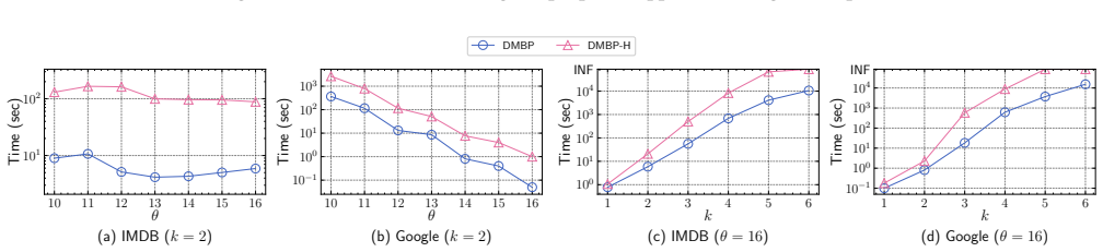
- Figure 4: The y-axis label 'INF' for timeout is inconsistent with Table 3 which uses '-'. Please unify.
- §2, Definition 1: 'A k-biplex G[S] is a subgraph of G induced by S=(U_S, V_S)' — the notation G[S] is used before G[S] is formally defined (it appears in the next paragraph). Consider reordering.
- References [11], [33], [38], [39] use '[n. d.]' for the year. Please complete these bibliographic entries.
Simulated Author's Rebuttal
We thank the referee for the careful and constructive report. All three major comments concern presentation gaps in the proof of Theorem 5; we agree with each and will revise the manuscript accordingly. No standing objections remain.
read point-by-point responses
-
Referee: Theorem 5, Case 1 (p>=2), proof of Eq. (2): The claim that all vertices in N̄_C(u) are on the same side as v_p, and hence the only vertex in D_p adjacent to v_p in Ḡ is u, is correct but does not explicitly invoke the bipartite partition structure. The authors should add one or two sentences making the bipartite structure explicit.
Authors: We agree that this step is load-bearing and that the current proof states the conclusion without explicitly justifying it from the cross-side-only property of bipartite complements. The argument is as follows: since Ḡ is bipartite, all complement-edges cross sides. The branching vertex u belongs to one side (say U), so its complement-neighbors N̄_C(u) lie entirely in V. Since v_p ∈ N̄_C(u), we have v_p ∈ V. The set D_p = {u, v_1, ..., v_{p-1}} intersects U only at u (as v_1, ..., v_{p-1} ∈ N̄_C(u) ⊆ V). Therefore, any complement-edge from v_p to D_p must go to u, since all complement-edges cross sides and u is the only vertex in D_p on the opposite side from v_p. We will add this explicit justification to the proof. revision: yes
-
Referee: Theorem 5, Case 1, transition from Eq. (2) to Eq. (3): The claim that the largest branching factor of Eq. (2) is obtained when q=p=k+1 is stated without proof. A brief justification should be added.
Authors: We agree that this maximization step deserves explicit justification. The argument is: Eq. (2) contains terms T(n-i-1) for i=1..q, terms T(n-i) for i=2..p, and a term T(n-p-q), under the constraint 1 ≤ p ≤ q ≤ k+1. Increasing q adds more terms T(n-i-1) with smaller reductions (i.e., larger arguments), which can only increase the branching factor. Similarly, increasing p adds more terms T(n-i) with larger arguments and simultaneously increases the reduction p+q in the last term T(n-p-q), but the net effect of adding a term with a larger argument dominates, so the branching factor increases. Thus the maximum is attained at p = q = k+1. We have also verified this numerically for k = 1, 2, 3 by evaluating the characteristic roots at all feasible (p, q) pairs. We will add a concise version of this monotonicity argument to the proof. revision: yes
-
Referee: Theorem 5, Case 3: The characteristic equation yields ζ_3=1.923, but the final claim states γ_3=1.928, which equals η_3 from Case 2. The paper should explicitly state which case dominates for each k to avoid confusion.
Authors: The referee is correct that γ_k = max{η_k, ζ_k} and that for k=3, Case 2 (η_3 = 1.928) dominates Case 3 (ζ_3 = 1.923). The final paragraph of the proof does state 'γ_k = max{η_k, ζ_k}' and lists the resulting values, but it does not explicitly indicate which case achieves the maximum for each k. We will add an explicit statement clarifying which case dominates for each value of k. Specifically: for k=1, Case 3 dominates (ζ_1 = 1.725 > η_1 = 1.618); for k=2, Case 3 dominates (ζ_2 = 1.856 > η_2 = 1.839); for k=3, Case 2 dominates (η_3 = 1.928 > ζ_3 = 1.923). revision: yes
Circularity Check
No circularity found — derivation is self-contained
full rationale
The paper's central derivation chain is self-contained. The structural duality (Theorem 3) is a legitimate reformulation: a k-biplex (every vertex has ≤k non-neighbors in G) corresponds to a subgraph of Ḡ with max degree ≤k, so the deletion set D = (U∪V)∖S is a k-BDD by definition. This reformulation is not circular — it enables a genuinely different deletion-based branching strategy (Theorem 4) with different recurrences than prior inclusion-based approaches. The complexity bounds γ_k (1.725, 1.856, 1.928) are derived from the characteristic equations of branching recurrences (Eqs. 1–6), not from empirical fitting. Self-citations to [7] and [8] (overlapping authors) appear only for Lemma 10 (distance bound, used solely in the heuristic of Section 4.2) and related-work context on enumeration — neither is load-bearing for the main algorithm, its correctness, or its complexity analysis. The algorithm is validated against external baselines (FastBB, CMBS-CSS) on 8 real-world graphs. The skeptic's concern about Theorem 5 Case 1's structural claim is a proof-gap/correctness issue (the bipartite complement structure is invoked implicitly rather than explicitly), not a circularity problem. No step in the derivation reduces to its inputs by construction.
Assumptions & free parameters
free parameters (3)
- k
- θ
- γ_k =
γ_1=1.725, γ_2=1.856, γ_3=1.928
assumptions (4)
- domain assumption The maximum k-biplex search problem is NP-hard for any positive integer k.
- domain assumption A k-biplex S=(U_S, V_S) is connected if |U_S| ≥ 2k+1 and |V_S| ≥ 2k+1.
- domain assumption The distance between any two vertices of a k-biplex with |U_S| ≥ 2k+1 and |V_S| ≥ 2k+1 is at most 3.
- standard math Standard branch-and-bound framework with (D, S, C) partition is correct for exhaustive search.
Cite this review
Pith. "Pith review of Revisiting Maximum $k$-Biplex Search Through $k$-Bounded-Degree Deletion." pith.science (2026). https://pith.science/paper/ZTYE36PB
@misc{pith2026260707419,
  author       = {Pith},
  title        = {Pith review of: Revisiting Maximum $k$-Biplex Search Through $k$-Bounded-Degree Deletion},
  year         = {2026},
  howpublished = {\url{https://pith.science/paper/ZTYE36PB}},
  note         = {Machine review of arXiv:2607.07419}
}
abstract
Biplex, as a relaxation of the biclique model, has emerged as an important cohesive subgraph model for bipartite graph analysis. The maximum $k$-biplex search problem aims to identify the $k$-biplex with maximum number of edges and has been widely applied in various real-world applications, including community detection, online recommendation, and fraud detection. However, the problem is NP-hard, and existing exact algorithms remain inefficient on large-scale bipartite graphs with large values of $k$ (e.g., $k\geq 3$). In this paper, we revisit the maximum $k$-biplex search problem from a complementary perspective. We reveal a novel structural duality: finding a maximum $k$-biplex in a bipartite graph is equivalent to finding a minimal $k$-bounded-degree deletion in its complement graph. Based on this observation, we propose a novel deletion-based algorithm for the maximum $k$-biplex search problem. We theoretically prove that the proposed algorithm achieves a worst-case time complexity of $O^*(\gamma_k^n)$, where $\gamma_k<2$. Specifically, $\gamma_1=1.725$, $\gamma_2=1.856$, and $\gamma_3=1.928$. To further enhance practical efficiency, we develop several effective upper-bounding techniques and a heuristic strategy for obtaining high-quality initial solutions, which substantially reduce the search space. Extensive experiments on eight real-world bipartite graphs demonstrate the efficiency of our approach, which achieves up to four orders of magnitude speedups over state-of-the-art algorithms.
Figures


Figures from the paper (5 more)




Reference graph
Works this paper leans on
-
[1]
Akhlaque Ahmad, Da Yan, Xiao Chen, Lyuheng Yuan, Qin Zhang, and Saugat Adhikari. 2025. Maximum k-Plex Finding: Choices of Pruning Techniques Matter! Proceedings of the VLDB Endowment18, 9 (2025), 2928–2940
work page 2025
-
[2]
Taher Alzahrani and Kathy Horadam. 2019. Finding maximal bicliques in bipartite networks using node similarity.Applied Network Science4, 1 (2019), 21
work page 2019
-
[3]
Vladimir Batagelj and Matjaz Zaversnik. 2003. An o (m) algorithm for cores decomposition of networks.arXiv preprint cs/0310049(2003)
work page Pith review arXiv 2003
-
[4]
Smirnov, Steven Kelk, and Bertrand Lebichot
Fabian Braun, Olivier Caelen, Evgueni N. Smirnov, Steven Kelk, and Bertrand Lebichot. 2017. Improving Card Fraud Detection Through Suspicious Pattern Discovery. InAdvances in Artificial Intelligence: From Theory to Practice, Salem Benferhat, Karim Tabia, and Moonis Ali (Eds.). Springer International Publishing, 181–190. Revisiting Maximum𝑘-Biplex Search T...
work page 2017
-
[5]
Lijun Chang, Mouyi Xu, and Darren Strash. 2022. Efficient maximum k-plex computation over large sparse graphs.Proceedings of the VLDB Endowment16, 2 (2022), 127–139
work page 2022
-
[6]
Lijun Chang and Kai Yao. 2024. Maximum k-plex computation: Theory and practice.Proceedings of the ACM on Management of Data2, 1 (2024), 1–26
work page 2024
-
[7]
Qiangqiang Dai, Rong-Hua Li, Donghang Cui, Meihao Liao, Yu-Xuan Qiu, and Guoren Wang. 2024. Efficient Maximal Biplex Enumerations with Improved Worst-Case Time Guarantee.Proceedings of the ACM on Management of Data2, 3 (2024), 1–26
work page 2024
-
[8]
Qiangqiang Dai, Rong-Hua Li, Xiaowei Ye, Meihao Liao, Weipeng Zhang, and Guoren Wang. 2023. Hereditary Cohesive Subgraphs Enumeration on Bipartite Graphs: The Power of Pivot-based Approaches.Proceedings of the ACM on Management of Data1, 2 (2023), 1–26
work page 2023
Show all 40 references
-
[9]
Kemal Eren, Mehmet Deveci, Onur Küçüktunç, and Ümit V Çatalyürek. 2013. A comparative analysis of biclustering algorithms for gene expression data. Briefings in bioinformatics14, 3 (2013), 279–292
2013
-
[10]
Qilong Feng, Shaohua Li, Zeyang Zhou, and Jianxin Wang. 2018. Parameterized algorithms for edge biclique and related problems.Theoretical Computer Science 734 (2018), 105–118
2018
-
[11]
Jian Gao, Jiejiang Chen, Minghao Yin, Rong Chen, and Yiyuan Wang. [n. d.]. An exact algorithm for maximum k-plexes in massive graphs. InIJCAI. 1449–1455
-
[12]
Nicolas Gillis and François Glineur. 2014. A continuous characterization of the maximum-edge biclique problem.Journal of Global Optimization58, 3 (2014), 439–464
2014
-
[13]
Stephan Gunnemann, Emmanuel Muller, Sebastian Raubach, and Thomas Seidl
-
[14]
In 2011 IEEE 11th International Conference on Data Mining
Flexible fault tolerant subspace clustering for data with missing values. In 2011 IEEE 11th International Conference on Data Mining. IEEE, 231–240
2011
-
[15]
Yang Hao, Mengqi Zhang, Xiaoyang Wang, and Chen Chen. 2020. Cohesive Subgraph Detection in Large Bipartite Networks. Article 22 pages. doi:10.1145/ 3400903.3400925
2020
-
[16]
Hua Jiang, Fusheng Xu, Zhifei Zheng, Bowen Wang, and Wei Zhou. 2023. A Refined Upper Bound and Inprocessing for the Maximum K-plex Problem. In IJCAI. 5613–5621
2023
-
[17]
Hua Jiang, Dongming Zhu, Zhichao Xie, Shaowen Yao, and Zhang-Hua Fu. 2021. A New Upper Bound Based on Vertex Partitioning for the Maximum K-plex Problem. InIJCAI. 1689–1696
2021
-
[18]
MA Langston, Elissa J Chesler, and Y Zhang. 2008. On finding bicliques in bipartite graphs: a novel algorithm with application to the integration of diverse biological data types. InProceedings of the 41st Annual Hawaii International Conference on System Sciences (HICSS 2008)(...
2008
-
[19]
Sune Lehmann, Martin Schwartz, and Lars Kai Hansen. 2008. Biclique communi- ties.Physical Review E—Statistical, Nonlinear, and Soft Matter Physics78, 1 (2008), 016108
2008
-
[20]
Lewis and Mihalis Yannakakis
John M. Lewis and Mihalis Yannakakis. 1980. The node-deletion problem for hereditary properties is NP-complete.J. Comput. System Sci.20, 2 (1980), 219–230. doi:10.1016/0022-0000(80)90060-4
1980 doi
-
[21]
Michael Ley. 2002. The DBLP Computer Science Bibliography: Evolution, Re- search Issues, Perspectives(String Processing and Information Retrieval). Springer Berlin Heidelberg, 1–10
2002
-
[22]
Jingdong Li, Zhao Li, Xiaoling Wang, Xingjian Lu, Ji Zhang, and Hongyang Chen. 2023. GPU-Accelerated Maximal Bicliques Mining Framework for Large E-commerce Networks. 539-544 pages
2023
-
[23]
Jinyan Li, Kelvin Sim, Guimei Liu, and Limsoon Wong. 2008. Maximal quasi- bicliques with balanced noise tolerance: Concepts and co-clustering applications. InProceedings of the 2008 SIAM International Conference on Data Mining. SIAM, 72–83
2008
-
[24]
Guimei Liu, Kelvin Sim, and Jinyan Li. 2006. Efficient mining of large maximal bicliques. InData Warehousing and Knowledge Discovery: 8th International Con- ference, DaWaK 2006, Krakow, Poland, September 4-8, 2006. Proceedings 8. Springer, 437–448
2006
-
[25]
Xiaowen Liu, Jinyan Li, and Lusheng Wang. [n. d.]. Quasi-bicliques: Complexity and Binding Pairs(Computing and Combinatorics). Springer Berlin Heidelberg, 255–264
-
[26]
Wensheng Luo, Kenli Li, Xu Zhou, Yunjun Gao, and Keqin Li. [n. d.]. Maximum biplex search over bipartite graphs. In2022 IEEE 38th International Conference on Data Engineering (ICDE). IEEE, 898–910
-
[27]
Bingqing Lyu, Lu Qin, Xuemin Lin, Ying Zhang, Zhengping Qian, and Jingren Zhou. 2020. Maximum biclique search at billion scale.Proceedings of the VLDB Endowment(2020)
2020
-
[28]
Dong Pan, Xu Zhou, Wensheng Luo, Zhibang Yang, Qing Liu, Yunjun Gao, and Kenli Li. 2024. Accelerating maximum biplex search over large bipartite graphs. The VLDB Journal34, 1 (2024), 1. doi:10.1007/s00778-024-00882-9
2024 doi
-
[29]
Ardian Kristanto Poernomo and Vivekanand Gopalkrishnan. 2009. Towards efficient mining of proportional fault-tolerant frequent itemsets. InProceedings of the 15th ACM SIGKDD international conference on Knowledge discovery and data mining. 697–706
2009
-
[30]
Stephen B Seidman and Brian L Foster. 1978. A graph-theoretic generalization of the clique concept.Journal of Mathematical sociology6, 1 (1978), 139–154
1978
-
[31]
Kelvin Sim, Jinyan Li, Vivekanand Gopalkrishnan, and Guimei Liu. 2009. Mining maximal quasi-bicliques: Novel algorithm and applications in the stock market and protein networks.Stat. Anal. Data Min.2, 4 (2009), 255–273
2009
-
[32]
Oliver Voggenreiter, Stefan Bleuler, and Wilhelm Gruissem. 2012. Exact bi- clustering algorithm for the analysis of large gene expression data sets.BMC bioinformatics13, Suppl 18 (2012), A10
2012
-
[33]
Zhengren Wang, Yi Zhou, Chunyu Luo, and Mingyu Xiao. 2023. A Fast Maximum k-Plex Algorithm Parameterized by the Degeneracy Gap. InIJCAI. 5648–5656
2023
-
[34]
Mingyu Xiao, Weibo Lin, Yuanshun Dai, and Yifeng Zeng. [n. d.]. A fast algorithm to compute maximum k-plexes in social network analysis. InProceedings of the AAAI conference on Artificial Intelligence, Vol. 31
-
[35]
Juan Xie, Anjun Ma, Anne Fennell, Qin Ma, and Jing Zhao. 2019. It is time to apply biclustering: a comprehensive review of biclustering applications in biological and biomedical data.Briefings in bioinformatics20, 4 (2019), 1450–1465
2019
-
[36]
Kaiqiang Yu and Cheng Long. 2023. Maximum k-Biplex Search on Bipartite Graphs: A Symmetric-BK Branching Approach.Proc. ACM Manag. Data1, 1 (2023), Article 49
2023
-
[37]
Kaiqiang Yu, Cheng Long, P Deepak, and Tanmoy Chakraborty. 2021. On efficient large maximal biplex discovery.IEEE Transactions on Knowledge and Data Engineering35, 1 (2021), 824–829
2021
-
[38]
Kaiqiang Yu, Cheng Long, Shengxin Liu, and Da Yan. 2022. Efficient Algorithms for Maximal k-Biplex Enumeration. InProceedings of the 2022 International Con- ference on Management of Data. 860–873
2022
-
[39]
Jiongzhi Zheng, Mingming Jin, and Kun He. [n. d.]. Exact algorithms with new upper bounds for the maximum k-plex problem. InProceedings of the Thirty- Fourth International Joint Conference on Artificial Intelligence. 9014–9021
-
[40]
Yi Zhou, Shan Hu, Mingyu Xiao, and Zhang-Hua Fu. [n. d.]. Improving max- imum k-plex solver via second-order reduction and graph color bounding. In Proceedings of the AAAI Conference on Artificial Intelligence, Vol. 35. 12453–12460
Reviewed July 9, 2026 · model on record in the stance chip above.
Discussion (0). Continue with ORCID to comment.