Blending of Probability and Non-Probability Samples: Applications to a Survey of Military Caregivers

Bonnie Ghosh-Dastidar; Michael W. Robbins; Rajeev Ramchand

REVIEW 3 major objections 5 minor 54 references

Blending of Probability and Non-Probability Samples: Applications to a Survey of Military Caregivers

T0 review · 3 major / 5 minor · reviewed 2026-08-14 · deepseek-v4-flash

Challenge this review Re-run · record.json Download PDF Read on arXiv ↗ Review JSON

Pith's one-line read Blending a small probability sample with a convenience sample yields unbiased, more precise estimates of a rare subpopulation, and the method shows post-9/11 military caregivers have significantly higher depression.

desk verdict A useful, honest blending-methods paper with a fixable overclaim and an ignorability assumption that deserves a power analysis before the headline era effect is taken at face value. read the letter →

arxiv 1908.04217 v1 pith:ZZHAEZ6M submitted 2019-08-12 stat.ME

Michael W. Robbins , Bonnie Ghosh-Dastidar , Rajeev Ramchand This is my paper · ORCID

classification stat.ME MSC 62D05

keywords probabilitysamplenon-probabilityconveniencepropensityscoreweightingcalibrationblendedestimationmilitarycaregiverssurvey

verification ladder T0 review T1 audit T2 compute T3 formal

The pith

A machine-rendered reading of the paper's core claim, the machinery that carries it, and where it could break.

The reading

When a rare subpopulation is the target, a probability sample may be too small to produce precise estimates, while a convenience sample is large but potentially biased. The paper develops weighting methods, propensity-score and calibration, in both disjoint and simultaneous versions, that combine the two samples into one representative dataset, and proves that under five stated assumptions the resulting ratio estimators are unbiased for the population mean and more precise than the probability sample alone. In the motivating survey of military caregivers, only 72 post-9/11 caregivers came from the probability panel; adding 281 caregivers from a Wounded Warrior Project convenience sample and applying the weights sharpens the estimate of the depression gap between post-9/11 and pre-9/11 caregivers enough to reach statistical significance with two of the three weighting schemes. The paper's simulations show the method's limits: if selection into the convenience sample depends on the outcome or a latent correlate, blending can be less accurate than ignoring the convenience sample altogether.

What carries the argument

The central object is the propensity score $\gamma_i = P(S_2 \mid S_1 \cup S_2, x_i)$, the probability that a sampled unit belongs to the convenience sample given the combined sample and the auxiliary variables. Solving $\gamma_i = q_i/(d_i + q_i)$ for the convenience inclusion probability yields $q_i = d_i \gamma_i/(1-\gamma_i)$ for disjoint weighting, and adding $q_i$ to $d_i$ yields the blended inclusion probability $p_i = d_i/(1-\gamma_i)$ for simultaneous weighting. Inverse probability weights built from these expressions carry the argument, and the same setup supports the adequacy-of-blending test, which regresses the outcome on a sample indicator under disjoint weights. Calibration weighting is presented as an alternative that solves the benchmark equations directly, and a delete-a-group jackknife is recommended for variance estimation.

What would settle it

An independent probability-based sample of post-9/11 caregivers large enough to estimate the covariate-adjusted depression gap precisely would settle it: if its confidence interval excluded the blended estimates around 1.9–2.1, the ignorability assumption would be false. A cheaper check is a sensitivity analysis that adds a plausible unmeasured confounder correlated with both WWP membership and depression to the propensity model and asks whether the era coefficient loses significance.

Watch

Extended reading notes

Core claim

Under the paper's Assumptions 1–5, the unobservable inclusion probabilities for the convenience and blended samples can be recovered from the propensity score $\gamma_i = P(S_2 \mid S_1 \cup S_2, x_i)$. The identities $q_i = d_i \gamma_i/(1-\gamma_i)$ and $p_i = d_i/(1-\gamma_i)$ give, respectively, the convenience inclusion probability and the blended inclusion probability, so inverse-probability weights of the form $1/q_i$ or $1/p_i$ produce unbiased ratio estimators of the population mean (Assumption 5 is not needed for simultaneous weighting). Blending lowers variance relative to the probability sample alone, and the synthetic-data study shows the precision gain shrinks as the auxiliary variables become more strongly related to the outcome. In the caregiver application, the era-of-service coefficient in the depression regression is 1.93 with disjoint propensity weighting ($p = 0.0063$) and 2.14 with simultaneous calibration ($p = 0.0094$), whereas the probability sample alone gives 1.51 ($p = 0.1078$); the blended analyses thus support the conclusion that post-9/11 caregivers have higher depression after controlling for covariates.

Load-bearing premise

The load-bearing premise is that selection into the convenience sample is unrelated to the outcome once the measured auxiliary variables are controlled, because when that fails the simulations show every blending method has higher rMSE than the probability sample alone; a secondary fragile shortcut is the constant inclusion probability imputed to all 281 WWP cases, which enters the weights directly.

Editorial extensions

If this is right

For any rare subpopulation with a modest probability sample and a convenience sample, the formula $q_i = d_i \gamma_i/(1-\gamma_i)$ turns an estimable propensity score into a usable inclusion probability, so the convenience sample contributes weight without requiring its selection mechanism to be known.
In the caregiver application, simultaneous weighting (SPS and SC) gives smaller standard errors than disjoint weighting (DPS), making simultaneous weights the more efficient choice when the analyst does not need to test the adequacy of the auxiliary set.
The simulation settings where the outcome or a latent correlate drives convenience selection show that blending can increase rMSE over the probability sample alone, so the adequacy test is not merely diagnostic but load-bearing for the method's safety.
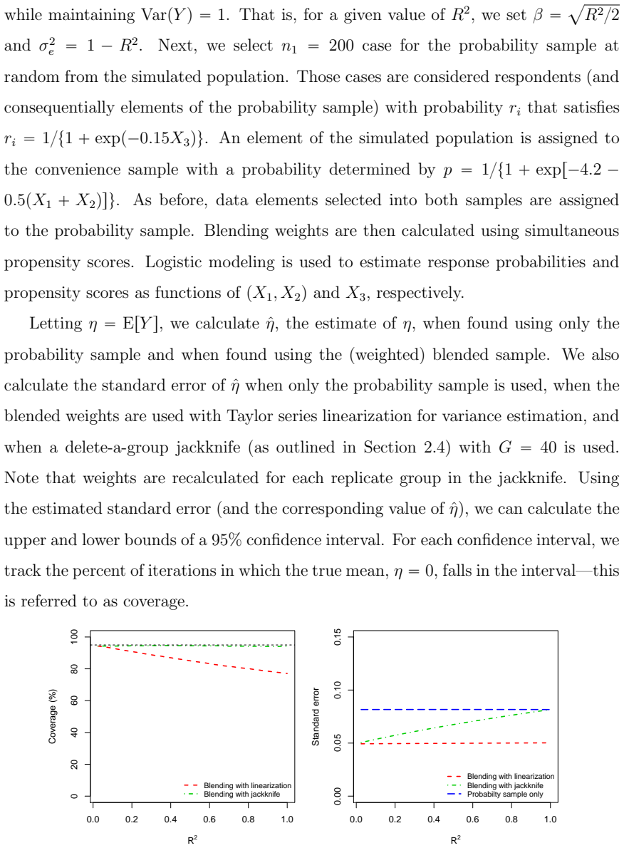
The R-squared study implies that researchers should avoid auxiliary variables that are strongly predictive of the outcome when the goal is variance reduction, because the convenience sample's precision contribution falls as the auxiliary-outcome association grows.
Variance estimation for blended estimators should rely on the jackknife rather than Taylor linearization when auxiliary-outcome associations are strong, since linearization coverage drops as R-squared increases.

Reading between the lines

Editorial extensions of the paper, not claims the author makes directly.

A natural extension is to give the adequacy test a calibrated power analysis: because the paper's support for Assumption 3 is non-rejection across 31 outcomes, quantifying how large a latent effect the test can detect would tell readers how much weight that non-rejection deserves.
The same identities should transfer to non-linear outcomes, such as binary indicators of caregiver burden, by replacing the linear adequacy regression with a logistic version, which the paper notes as an easy extension; the variance and bias behavior would need its own simulation check.
The paper's parsimony warning runs against conventional propensity-score advice to include outcome predictors; reconciling the two would give a principled variable-selection rule for blended samples, balancing bias control against lost precision.
A sensitivity analysis varying the constant inclusion probability imputed to all 281 WWP cases would show how much of the era-of-service effect depends on that shortcut; the paper acknowledges the shortcut but does not assess its impact.

Share X Bluesky LinkedIn Reddit HN

Signed reviews

No signed human review yet.

Editorial analysis

A structured set of objections, weighed in public.

Desk editor's note, referee report, and a circularity audit.

Desk Editor's Note

read the letter

Bottom line: this is a useful, honest survey-methods paper that deserves a serious referee, but the headline application claim is shakier than the prose suggests, and one significance statement is plainly wrong. The methods are not as new as the authors imply — the weights in (3) and (7) are straightforward algebra once you define gamma_i — but the paper organizes the alternatives (disjoint vs. simultaneous, propensity vs. calibration) clearly, and the simulation work is genuinely careful. Setting 1 shows all methods work when the ignorability assumption holds, and Settings 3–5 show they degrade when it fails, sometimes below the probability sample alone. That is the kind of honest stress-testing that applied work too often skips. The practical guidance is also sensible: simultaneous blending for precision, disjoint blending as the diagnostic tool, jackknife over linearization when R^2 is moderate, and parsimony in auxiliary variables. For a survey-methods audience, the paper is a clear recipe, even if not a deep theoretical advance.

The soft spots are real but fixable. First, Section 3.3.3 claims all blending methods reach 5% significance for the era effect, but Table 5 gives SPS p = 0.078. That is an overclaim and it is internally inconsistent. Second, the propensity weights for the WWP rest on a constant inclusion probability d_i imputed to all 281 cases, with no sensitivity analysis. Third, and most important, the application's validity rests on Assumption 3 (ignorability): selection into the WWP is independent of depression given covariates. The only empirical support is non-rejection of the adequacy test across 31 outcomes. The stress-test note makes a fair point: the paper's own Table 7 shows that test has rejection rates only 0.47 and 0.23 under simulated violations (Settings 4 and 5), and in those settings blending makes rMSE worse than probability-only. So a true violation of the size simulated would often go undetected, and the era coefficient shifting from 1.51 to 1.68–2.14 could in principle be a latent confounder (e.g., anxiety) rather than a real era effect. The authors acknowledge the test's power only implicitly. That does not sink the paper, but it should be addressed directly.

Who is this for? Survey practitioners who need to blend rare-population convenience samples with probability samples and want a well-documented recipe with honest failure modes. It is not a theoretical breakthrough, but it is a solid applied methodology paper. I would send it to a serious referee and expect acceptance after fixing the overclaim, adding a sensitivity analysis for d_i, and ideally a power or minimum-detectable-bias analysis for the adequacy test.

Referee Report

3 major / 5 minor

Summary. The manuscript develops weighting estimators that combine a probability sample with a convenience sample from the same target population. Two propensity-score weighting schemes are derived: disjoint weights based on q_i = d_i gamma_i/(1-gamma_i) (Eq. 3) and simultaneous weights based on p_i = d_i/(1-gamma_i) (Eq. 7), together with disjoint and simultaneous calibration weights. The authors also propose a test for the adequacy of blending based on comparing weighted estimates from the two samples (Eqs. 10-11) and discuss jackknife versus linearization variance estimation. The methods are applied to a RAND military-caregiver survey with 72 post-9/11 caregivers from KnowledgePanel and 281 from the Wounded Warrior Project. The regression of depression on era and covariates (Eq. 13) gives a positive era coefficient that is significant under disjoint propensity scores and simultaneous calibration but not under KnowledgePanel-only or simultaneous propensity scores. Simulation studies with a caregiver pseudo-population and with synthetic data evaluate bias, root mean squared error, design effects, rejection rates, and variance-estimator coverage under five selection settings.

Significance. The paper is a serious contribution to the modest literature on blending probability and convenience samples. The derivations of Eqs. (3) and (7) are straightforward, and the simulation design is unusually honest: Setting 1 validates the methods against a known mechanism, Settings 3-5 quantify degradation under ignorability failures, and Section 4.2 demonstrates that linearization under-covers when auxiliary variables are strongly related to the outcome while a delete-a-group jackknife maintains coverage. If the assumptions hold, the proposed weights offer practical tools for rare subpopulations. The main unresolved issue is not internal consistency but the strength of evidence for Assumption 3 in the application, on which the headline era-effect finding depends.

major comments (3)

[Section 2.3, Table 7] The only empirical support for Assumption 3 in the application is non-rejection of the adequacy test (11) for all 31 outcomes; however, the paper's own Table 7 shows that at tau = 1/2 the test rejects only 47% of the time (DPS, Setting 4) and 23% of the time (DPS, Setting 5) when ignorability is violated, and in those settings blending either degrades or does not clearly improve on the probability sample alone (e.g., Setting 4 rMSEs 14.3-17.6 versus 11.6 for KP-only). The application therefore needs a power or minimum-detectable-bias analysis for the adequacy test at the observed effective sample sizes, and a sensitivity check showing what size of unobserved confounding would change the era coefficient eta_1 in Eq. (13). As written, the statement in Section 5 that Assumption 3 'appears upheld' is weaker than the evidence supports.
[Section 3.3.1, Eqs. (3), (7)] The imputation d_i = n1 / sum_{j in S1} d_j^{-1} for all i in S2 assumes equal probability of inclusion into the KnowledgePanel for WWP cases. This assumption enters directly into the propensity-based weights through q_i in Eq. (3) and p_i in Eq. (7). The paper acknowledges the shortcut but does not quantify its effect on the estimated means or on eta_1 in Eq. (13). A sensitivity analysis that perturbs d_i over a plausible range, or that compares propensity-based estimates with calibration estimates that do not require d_i for S2, is needed to establish that the DPS and SC results in Table 5 are not artifacts of this imputation.
[Section 4.2, Table 5] The simulation in Section 4.2 shows that Taylor-series linearization under-covers when R^2 between the auxiliary variables and the outcome is moderate or high, whereas the delete-a-group jackknife maintains coverage. The application section states that sample means and regression results are computed with svymean() and svyglm() (Section 3.3.3), whose default variance estimators are linearization-based. Since the auxiliary variables in Tables 2-3 are strongly associated with depression, the p-values 0.0063 (DPS) and 0.0094 (SC) for eta_1 in Eq. (13) may be optimistic. The authors should report jackknife-based standard errors and p-values for the regression coefficients, or at least assess R^2 for the model in Eq. (13) and establish that the linearization-based results fall in a regime where coverage is adequate.

minor comments (5)

[Section 3.3.3] The sentence 'disjoint blending yields larger standard errors ... and is not evidence of a loss of precision' is misleading: a larger standard error is, by definition, evidence of lower precision. The intended point about bias-variance trade-off should be stated more carefully.
[Section 3.3.3] The explanation that simultaneous weights yield small p-values for the adequacy test because they make the samples individually non-representative is correct but could be stated before Table 4; otherwise readers may misinterpret those p-values.
[Eq. (12)] The notation p zeta0, zeta1 q' should be written as (zeta0, zeta1)' to distinguish the vector of regression parameters from a probability.
[Section 4.1, Table 6] The table entries for 'Caregiver depression' and 'Caregiver anxiety' mix a numeric coefficient with an asterisk in a way that is easy to misread; a cleaner format would separate the two pieces.
[Section 5] The statement that Assumption 3 'appears upheld' because the adequacy test did not reject should explicitly cite the low power demonstrated in Table 7, rather than treating non-rejection as confirmation.

Circularity Check

0 steps flagged · score 1.0 of 10

No significant circularity: the weight formulas are algebraic identities, the era-effect estimate is not fitted from the outcome, and the self-citations are not load-bearing.

full rationale

The paper's central derivations are self-contained. The weight formulas (3) and (7), q_i = d_i gamma_i/(1-gamma_i) and p_i = d_i/(1-gamma_i), follow algebraically from the definition gamma_i = P(S2|S1 U S2, x_i) and the disjointness of S1 and S2; the unbiasedness claims are standard Horvitz-Thompson arguments under Assumptions 1-3 and 5, not restatements of fitted outputs. The propensity score and nonresponse models are estimated nuisance parameters that are then plugged into the weights; this is a standard two-step procedure, and the paper validates it against external simulation benchmarks with known selection mechanisms, including settings where the assumptions fail (Table 7). The headline application result, the era coefficient eta_1 in Eq. (13), is not forced by construction: the outcome DEP is not among the auxiliary variables used to estimate gamma_i or the calibration benchmarks, so the significant eta_1 under DPS and SC is an empirical consequence rather than a fitted input. The self-citations are not load-bearing: Ramchand et al. (2014) supplies the external survey data, and Robbins et al. (2017) supports a secondary distance-metric choice that does not determine unbiasedness. The adequacy test's low power, visible in the paper's own Table 7 Settings 4-5, weakens the empirical support for Assumption 3, but that is a correctness or inferential risk, not a circular derivation step.

Assumptions & free parameters 5 free parameters · 8 assumptions · 0 invented entities

Everything the central claim rests on is either a standard survey-design quantity or one of the five numbered assumptions in Section 2.1. No new entities are postulated. The estimator-relevant fitted quantities are the propensity and nonresponse model coefficients plus the data-determined constants kappa and weight-trimming bounds. Assumption 3 (ignorability of the convenience sample) is the fragile one, and its failure is shown in the paper's own Settings 3-5 to make blending harmful.

free parameters (5)

Propensity score logistic coefficients zeta0, zeta1 (Eq. 12) = not reported numerically
gamma_i is replaced by fitted values from a logistic regression on the auxiliary variables; all blended weights inherit these fitted inclusion probabilities.
Constant inclusion probability d_i for WWP cases = n1 / sum_{j in S1} d_j^{-1}; constant, value not reported
Every one of the 281 WWP cases is assigned the same probability of inclusion in the probability sample; enters the SPS and DPS weights directly.
Blend constant kappa for disjoint weights = data-determined from Kish deff formula; not reported
kappa splits emphasis between the two samples; chosen to minimize the Kish approximation of the design effect rather than the true variance.
Weight trimming bounds = top and bottom 1% truncated
Extreme weights are truncated at the 1st and 99th percentiles and remaining weights adjusted to preserve the sum; affects benchmark alignment in Table 3.
Simulation tuning parameter tau (Table 6, Settings 3-5) = 1/2
Controls the strength of outcome-dependent selection into the convenience sample; fixed at 1/2 in the main text and varied in the supplement. A simulation design choice, not an estimator input.

assumptions (8)

domain assumption Assumption 1: selection probabilities for S1* depend only on design variables x*_i, are known, and are positive
Required so that d*_i is known for all units in S1* union S2. Reasonable for a designed panel, but the KP screener details are proprietary and partially unobservable.
domain assumption Assumption 2: nonresponse in S1* is missing at random given rxi, with estimable response probabilities r_i > 0
In the application the authors cannot estimate r_i for WWP cases (Section 3.3.1), so they substitute a constant d_i; this is a self-acknowledged relaxation.
domain assumption Assumption 3: ignorability for the convenience sample, P(S2|x_i,y_i) = P(S2|x_i)
The load-bearing premise. The paper's own simulations (Settings 4-5, Table 7) show every blending method becomes more biased than the probability sample alone when this fails. In the application, WWP caregivers volunteer through an advocacy organization, so outcome-driven selection is plausible.
domain assumption Assumption 4: the models for r_i and gamma_i are correctly specified
The paper itself notes (Section 5) that in its simulations the logistic propensity model is misspecified relative to the true drawing mechanism, and that the methods still perform acceptably.
domain assumption Assumption 5: positivity of the convenience sample, q_i > 0 for all i
Needed for disjoint blending only; simultaneous weights do not require coverage, an advantage the paper highlights.
domain assumption The probability and convenience samples are disjoint
Used to write gamma_i = q_i/(d_i + q_i). In simulations, double selections are assigned to the probability sample (Section 4.1).
domain assumption Unstratified, unclustered design for the main theory
The paper states this is for expository simplicity and claims extension to stratified and clustered designs in Section 5, but the formal results are presented only for the simple design.
ad hoc to paper All WWP cases had equal probability of inclusion in the KnowledgePanel (constant d_i for S2)
The substitution d_i = n1/sum_{j in S1} d_j^{-1} (Section 3.3.1) is a modeling shortcut forced by the proprietary screener data; it affects SPS and DPS weights in the application.

how reviews work

0 comments

Cite this review

Pith. "Pith review of Blending of Probability and Non-Probability Samples: Applications to a Survey of Military Caregivers." pith.science (2026). https://pith.science/paper/ZZHAEZ6M

@misc{pith2026190804217,
  author       = {Pith},
  title        = {Pith review of: Blending of Probability and Non-Probability Samples: Applications to a Survey of Military Caregivers},
  year         = {2026},
  howpublished = {\url{https://pith.science/paper/ZZHAEZ6M}},
  note         = {Machine review of arXiv:1908.04217}
}

read the original abstract

Probability samples are the preferred method for providing inferences that are generalizable to a larger population. However, when a small (or rare) subpopulation is the group of interest, this approach is unlikely to yield a sample size large enough to produce precise inferences. Non-probability (or convenience) sampling often provides the necessary sample size to yield efficient estimates, but selection bias may compromise the generalizability of results to the broader population. Motivating the exposition is a survey of military caregivers; our interest is focused on unpaid caregivers of wounded, ill, or injured servicemembers and veterans who served in the US armed forces following September 11, 2001. An extensive probability sampling effort yielded only 72 caregivers from this subpopulation. Therefore, we consider supplementing the probability sample with a convenience sample from the same subpopulation, and we develop novel methods of statistical weighting that may be used to combine (or blend) the samples. Our analyses show that the subpopulation of interest endures greater hardships than caregivers of veterans with earlier dates of service, and these conclusions are discernably stronger when blended samples with the proposed weighting schemes are used. We conclude with simulation studies that illustrate the efficacy of the proposed techniques, examine the bias-variance trade-off encountered when using inadequately blended data, and show that the gain in precision provided by the convenience sample is lower in circumstances where the outcome is strongly related to the auxiliary variables used for blending.

Figures

Figures reproduced from arXiv: 1908.04217 by the authors.

Discussion (0). Continue with ORCID to comment.

Reference graph

Works this paper leans on

54 extracted references · 48 canonical work pages

[1]

Baker, R., S. J. Blumberg, J. M. Brick, M. P. Couper, M. Courtright, J. M. Dennis, D. Dillman, M. R. Frankel, P. Garland, R. M. Groves, C. Kennedy, J. Krosnick, P. J. Lavrakas, S. Lee, M. Link, L. Piekarski, K. Rao, R. K. Thomas, and D. Zahs (2010). Research synthesis: AAPOR report on online panels. Public Opinion Quarterly\/ 74\/ (4), 711--781

work page 2010
[2]

Baker, R., J. M. Brick, N. A. Bates, M. Battaglia, M. P. Couper, J. A. Dever, K. J. Gile, and R. Tourangeau (2013). Report on the AAPOR Task Force on Non-Probability Sampling . American Association for Public Opinion Research

work page 2013
[3]

Cobben, and B

Bethlehem, J., F. Cobben, and B. Schouten (2011). The use of response propensities. In Handbook of Nonresponse in Household Surveys , pp.\ 327--352. John Wiley & Sons, Inc

work page 2011
[4]

Biffignandi, S. and J. Bethlehem (2012). Web surveys: Methodological problems and research perspectives. In Advanced Statistical Methods for the Analysis of Large Data-Sets , pp.\ 363--373. Springer

work page 2012
[5]

Blasius, J. and M. Brandt (2010). Representativeness in online surveys through stratified samples. Bulletin de M \'e thodologie Sociologique\/ 107\/ (1), 5--21

work page 2010
[6]

Brookhart, M. A., S. Schneeweiss, K. J. Rothman, R. J. Glynn, J. Avorn, and T. St \"u rmer (2006). Variable selection for propensity score models. American Journal of Epidemiology\/ 163\/ (12), 1149--1156

work page 2006
[7]

Chang, L. and J. A. Krosnick (2009). National surveys via RDD telephone interviewing versus the internet comparing sample representativeness and response quality. Public Opinion Quarterly\/ 73\/ (4), 641--678

work page 2009
[8]

and C.-E

Deville, J.-C. and C.-E. S \"a rndal (1992). Calibration estimators in survey sampling. Journal of the American Statistical Association\/ 87\/ (418), 376--382

work page 1992

Show all 54 references

[9]

S \"a rndal, and O

Deville, J.-C., C.-E. S \"a rndal, and O. Sautory (1993). Generalized raking procedures in survey sampling. Journal of the American Statistical Association\/ 88\/ (423), 1013--1020

1993
[10]

DiSogra, C., C. Cobb, E. Chan, and J. M. Dennis (2011, August). Calibrating non-probability internet samples with probability samples using early adopter characteristics. In JSM Proceedings , Alexandria, VA, pp.\ 4501--4515. Section on Survey Research Methods: American Statist...

2011
[11]

Smith, G

Duffy, B., K. Smith, G. Terhanian, and J. Bremer (2005). Comparing data from online and face-to-face surveys. International Journal of Market Research\/ 47\/ (6), 615

2005
[12]

Elliott, M. N. and A. Haviland (2007). Use of a web-based convenience sample to supplement a probability sample. Survey Methodology\/ 33\/ (2), 211--5

2007
[13]

Friedman, J. H. (2001). Greedy function approximation: A gradient boosting machine. Annals of Statistics\/ , 1189--1232

2001
[14]

Friedman, J. H. (2002). Stochastic gradient boosting. Computational Statistics & Data Analysis\/ 38\/ (4), 367--378

2002
[15]

Fr \"o lich, M. (2006). Non-parametric regression for binary dependent variables. The Econometrics Journal\/ 9\/ (3), 511--540

2006
[16]

KnowledgePanel Design Summary

GfK (2013). KnowledgePanel Design Summary . URL : www.knowledgenetworks.com/\ /docs/knowledgepanel\ Last accessed: January 2015

2013
[17]

Ghosh-Dastidar, B., M. N. Elliott, A. M. Haviland, and L. A. Karoly (2009). Composite estimates from incomplete and complete frames for minimum- MSE estimation in a rare population: An application to families with young children. Public Opinion Quarterly\/ 73\/ (4), 761--784

2009
[18]

Hahn, J. (1998). On the role of the propensity score in efficient semiparametric estimation of average treatment effects. Econometrica\/ , 315--331

1998
[19]

Hartley, H. O. (1974). Multiple frame methodology and selected applications. Sankhya, Series C\/ 36 , 99--118

1974
[20]

Hirano, K., G. W. Imbens, and G. Ridder (2003). Efficient estimation of average treatment effects using the estimated propensity score. Econometrica\/ 71\/ (4), 1161--1189

2003
[21]

Horvitz, D. G. and D. J. Thompson (1952). A generalization of sampling without replacement from a finite universe. Journal of the American Statistical Association\/ 47\/ (260), 663--685

1952
[22]

Kish, L. (1965). Survey Sampling . New York, NY: John Wiley and Sons

1965
[23]

Kott, P. S. (2001). The delete-a-group jackknife. Journal of Official Statistics\/ 17\/ (4), 521

2001
[24]

Kott, P. S. (2006). Using calibration weighting to adjust for nonresponse and coverage errors. Survey Methodology\/ 32\/ (2), 133

2006
[25]

Kott, P. S. and F. A. Vogel (1995). Multiple-frame business surveys. Business Survey Methods\/ , 185--203

1995
[26]

Kroenke, K., T. W. Strine, R. L. Spitzer, J. B. Williams, J. T. Berry, and A. H. Mokdad (2009). The PHQ -8 as a measure of current depression in the general population. Journal of Affective Disorders\/ 114\/ (1), 163--173

2009
[27]

Lee, B. K., J. Lessler, and E. A. Stuart (2011). Weight trimming and propensity score weighting. PloS one\/ 6\/ (3), e18174

2011
[28]

Lee, S. (2006). Propensity score adjustment as a weighting scheme for volunteer panel web surveys. Journal of Official Statistics\/ 22\/ (2), 329

2006
[29]

Lee, S. and R. Valliant (2009). Estimation for volunteer panel web surveys using propensity score adjustment and calibration adjustment. Sociological Methods & Research\/ 37\/ (3), 319--343

2009
[30]

Little, R. J. A. and D. B. Rubin (2002). Statistical A nalysis with M issing D ata\/ (2nd ed.). New J ersey: John W iley & S ons

2002
[31]

Lohr, S. (2011). Alternative survey sample designs: Sampling with multiple overlapping frames. Survey Methodology\/ 37\/ (2), 197--213

2011
[32]

Lumley, T. (2004). Analysis of complex survey samples. Journal of Statistical Software\/ 9\/ (1), 1--19

2004
[33]

Lumley, T. (2011). Complex Surveys: A Guide to Analysis using R , Volume 565. John Wiley & Sons

2011
[34]

Merkouris, T. (2004). Combining independent regression estimators from multiple surveys. Journal of the American Statistical Association\/ 99\/ (468), 1131--1139

2004
[35]

Profile of post-9/11 veterans: 2012

NCVAS (2015). Profile of post-9/11 veterans: 2012. Technical report. URL : http://www.va.gov/vetdata/docs/SpecialReports/Post_911_Veterans_Profile_2012_July2015.pdf , L ast Accessed: 2015-07-15

2015
[36]

Potter, F. and Y. Zheng (2015). Methods and issues in trimming extreme weights in sample surveys. In Proceedings of the American Statistical Association, Section on Survey Research Methods , pp.\ 2707--2719

2015
[37]

Quenouille, M. H. (1949). Problems in plane sampling. The Annals of Mathematical Statistics\/ 20\/ (3), 355--375

1949
[38]

Quenouille, M. H. (1956). Notes on bias in estimation. Biometrika\/ 43\/ (3/4), 353--360

1956
[39]

Tanielian, M

Ramchand, R., T. Tanielian, M. P. Fisher, C. A. Vaughan, T. E. Trail, C. Epley, P. Voorhies, M. Robbins, E. Robinson, and B. Ghosh-Dastidar (2014). Hidden Heroes: America's Military Caregivers . Santa Monica, CA: RAND Corporation

2014
[40]

Rao, J. and C. Wu (2010). Pseudo--empirical likelihood inference for multiple frame surveys. Journal of the American Statistical Association\/ 105\/ (492), 1494--1503

2010
[41]

Renssen, R. H. and N. J. Nieuwenbroek (1997). Aligning estimates for common variables in two or more sample surveys. Journal of the American Statistical Association\/ 92\/ (437), 368--374

1997
[42]

McCaffrey, A

Ridgeway, G., D. McCaffrey, A. Morral, B. A. Griffin, and L. Burgette (2014). twang: Toolkit for Weighting and Analysis of Nonequivalent Groups . R package version 1.4-0

2014
[43]

Huggins, and D

Rivers, D., V. Huggins, and D. Slotwiner (2003, August). Combining random and non-random samples. In JSM Proceedings . American Statistical Association

2003
[44]

Robbins, M. W., J. Saunders, and B. Kilmer (2017). A framework for synthetic control methods with high-dimensional, micro-level data: Evaluating a neighborhood-specific crime intervention. Journal of the American Statistical Association\/ 112\/ (517), 109--126

2017
[45]

Rosenbaum, P. R. and D. B. Rubin (1983). The central role of the propensity score in observational studies for causal effects. Biometrika\/ 70\/ (1), 41--55

1983
[46]

S \"a rndal, C.-E. (2007). The calibration approach in survey theory and practice. Survey Methodology\/ 33\/ (2), 99--119

2007
[47]

Van Soest, and A

Schonlau, M., A. Van Soest, and A. Kapteyn (2007). Are `webographic' or attitudinal questions useful for adjusting estimates from web surveys using propensity scoring? Survey Research Methods\/ 1 , 155--163

2007
[48]

van Soest, A

Schonlau, M., A. van Soest, A. Kapteyn, and M. Couper (2009). Selection bias in web surveys and the use of propensity scores. Sociological Methods & Research\/ 37\/ (3), 291--318

2009
[49]

Zapert, L

Schonlau, M., K. Zapert, L. P. Simon, K. H. Sanstad, S. M. Marcus, J. Adams, M. Spranca, H. Kan, R. Turner, and S. H. Berry (2004). A comparison between responses from a propensity-weighted web survey and an identical RDD survey. Social Science Computer Review\/ 22\/ (1), 128--138

2004
[50]

Conrad, and M

Tourangeau, R., F. Conrad, and M. Couper (2013). The Science of Web Surveys . New York: Oxford University Press

2013
[51]

Valliant, R. and J. A. Dever (2011). Estimating propensity adjustments for volunteer web surveys. Sociological Methods & Research\/ 40\/ (1), 105--137

2011
[52]

Rothschild, S

Wang, W., D. Rothschild, S. Goel, and A. Gelman (2015). Forecasting elections with non-representative polls. International Journal of Forecasting\/ 31\/ (3), 980--991

2015
[53]

Yeager, D. S., J. A. Krosnick, L. Chang, H. S. Javitz, M. S. Levendusky, A. Simpser, and R. Wang (2011). Comparing the accuracy of RDD telephone surveys and internet surveys conducted with probability and non-probability samples. Public Opinion Quarterly\/ 75\/ (4), 709--747

2011
[54]

Zieschang, K. D. (1986). A generalized least squares weighting system for the consumer expenditure survey. In Proceedings of the Section on Survey Research Methods, American Statistical Association Meetings , pp.\ 64--71

1986

Pith tools

Reviewed August 14, 2026 · model on record in the stance chip above.

[1] [1]

Baker, R., S. J. Blumberg, J. M. Brick, M. P. Couper, M. Courtright, J. M. Dennis, D. Dillman, M. R. Frankel, P. Garland, R. M. Groves, C. Kennedy, J. Krosnick, P. J. Lavrakas, S. Lee, M. Link, L. Piekarski, K. Rao, R. K. Thomas, and D. Zahs (2010). Research synthesis: AAPOR report on online panels. Public Opinion Quarterly\/ 74\/ (4), 711--781

work page 2010

[2] [2]

Baker, R., J. M. Brick, N. A. Bates, M. Battaglia, M. P. Couper, J. A. Dever, K. J. Gile, and R. Tourangeau (2013). Report on the AAPOR Task Force on Non-Probability Sampling . American Association for Public Opinion Research

work page 2013

[3] [3]

Cobben, and B

Bethlehem, J., F. Cobben, and B. Schouten (2011). The use of response propensities. In Handbook of Nonresponse in Household Surveys , pp.\ 327--352. John Wiley & Sons, Inc

work page 2011

[4] [4]

Biffignandi, S. and J. Bethlehem (2012). Web surveys: Methodological problems and research perspectives. In Advanced Statistical Methods for the Analysis of Large Data-Sets , pp.\ 363--373. Springer

work page 2012

[5] [5]

Blasius, J. and M. Brandt (2010). Representativeness in online surveys through stratified samples. Bulletin de M \'e thodologie Sociologique\/ 107\/ (1), 5--21

work page 2010

[6] [6]

Brookhart, M. A., S. Schneeweiss, K. J. Rothman, R. J. Glynn, J. Avorn, and T. St \"u rmer (2006). Variable selection for propensity score models. American Journal of Epidemiology\/ 163\/ (12), 1149--1156

work page 2006

[7] [7]

Chang, L. and J. A. Krosnick (2009). National surveys via RDD telephone interviewing versus the internet comparing sample representativeness and response quality. Public Opinion Quarterly\/ 73\/ (4), 641--678

work page 2009

[8] [8]

and C.-E

Deville, J.-C. and C.-E. S \"a rndal (1992). Calibration estimators in survey sampling. Journal of the American Statistical Association\/ 87\/ (418), 376--382

work page 1992