REVIEW 1 major objections 2 minor 2 cited by
Bayesian modeling of nearly mutually orthogonal processes
T0 review · 1 major / 2 minor · reviewed 2026-05-24 · grok-4.3
Pith's one-line read Nearly mutually orthogonal processes enforce mutual orthogonality of functional factor loadings while preserving computational simplicity.
desk verdict The paper introduces a penalty-tuned construction for nearly mutually orthogonal processes to ease orthogonality constraints in functional factor analysis, but offers little evidence on whether it actually delivers the claimed efficiency without side effects. read the letter →
The pith
A machine-rendered reading of the paper's core claim, the machinery that carries it, and where it could break.
The reading
What carries the argument
Nearly mutually orthogonal processes, stochastic processes whose joint distribution incorporates a penalty parameter that encourages mutual orthogonality.
What would settle it
Compare posterior samples from the nearly orthogonal model against samples from an exactly orthogonal constrained model on the same dataset and check whether the loadings deviate substantially from orthogonality or whether predictive performance degrades.
Extended reading notes
Core claim
Nearly mutually orthogonal processes are stochastic processes whose joint distribution is governed by a penalty parameter that determines the degree to which the processes are mutually orthogonal; this construction allows the processes to be used as factor loadings in a functional factor model while maintaining computational simplicity and efficiency for Bayesian posterior inference.
Load-bearing premise
The penalty parameter trades off orthogonality against computational tractability without introducing substantial bias or loss of flexibility in the posterior.
Editorial extensions
If this is right
- The penalty parameter directly controls the achievable level of orthogonality in the factor loadings.
- Posterior computation remains straightforward because the processes avoid hard constraints.
- The resulting model supports interpretable inference on covariate effects in longitudinal functional data.
- The approach extends the range of functional factor models that can be fit in Bayesian settings without prohibitive cost.
Reading between the lines
- The construction could be adapted to enforce other linear constraints on loadings in non-functional factor models.
- In very high-dimensional settings the penalty might need calibration to avoid under- or over-constraining the factors.
- Simulations with known orthogonal loadings could quantify how close the posterior loadings come to exact orthogonality for different penalty values.
Editorial analysis
A structured set of objections, weighed in public.
Referee Report
Summary. The manuscript introduces nearly mutually orthogonal processes (NeMO) as a device for Bayesian functional factor analysis. These processes are defined via a joint distribution controlled by an explicit penalty parameter that encourages approximate mutual orthogonality of the functional factor loadings while preserving computational tractability for posterior sampling. The approach is illustrated through an application to longitudinal childhood weight data examining effects of breastfeeding status, illness, and demographic factors.
Significance. If the construction holds, the method supplies a practical route to interpretable factor loadings in functional data models without the computational burden of hard orthogonality constraints. The public GitHub code is a clear strength that aids reproducibility and adoption.
major comments (1)
- [Model definition and simulation study] The central modeling claim rests on the penalty parameter successfully trading off orthogonality against bias and flexibility in the posterior (reader's weakest assumption). The manuscript should include a targeted simulation study or sensitivity analysis quantifying how posterior inferences on loadings and factors change as the penalty varies across a range that spans near-orthogonality to near-independence.
minor comments (2)
- [Abstract] The abstract states that the method maintains efficiency but provides no quantitative metrics (e.g., runtime, effective sample size, or comparison to unconstrained FFA); adding one sentence summarizing such evidence would strengthen the claim.
- [Methods] Notation for the processes, the penalty, and the resulting covariance structure should be introduced with a short table or diagram in the methods section to aid readers new to functional factor models.
Simulated Author's Rebuttal
We thank the referee for their constructive review and positive recommendation for minor revision. We address the single major comment below and will incorporate the suggested addition in the revised manuscript.
read point-by-point responses
-
Referee: The central modeling claim rests on the penalty parameter successfully trading off orthogonality against bias and flexibility in the posterior (reader's weakest assumption). The manuscript should include a targeted simulation study or sensitivity analysis quantifying how posterior inferences on loadings and factors change as the penalty varies across a range that spans near-orthogonality to near-independence.
Authors: We agree that explicitly quantifying the effect of the penalty parameter via simulation would strengthen the presentation of the central modeling claim. In the revised manuscript we will add a targeted simulation study in which we generate data under the NeMO construction, vary the penalty across a grid spanning near-orthogonality to near-independence, and report the resulting changes in posterior summaries of the loadings and latent factors. This will directly illustrate the bias-flexibility trade-off and complement the existing real-data application. revision: yes
Circularity Check
No significant circularity detected
full rationale
The paper proposes nearly mutually orthogonal processes as an explicit modeling device controlled by a tunable penalty parameter that directly trades off orthogonality against posterior sampling ease. This construction is introduced as a deliberate modeling choice for functional factor analysis rather than a result derived from first principles or external theorems. No load-bearing self-citations, fitted inputs renamed as predictions, or self-definitional reductions appear in the provided abstract or described claims; the joint distribution is defined directly in terms of the penalty, and the application to childhood weight data serves as an illustration of the method rather than a validation that collapses into the modeling assumptions themselves. The derivation chain is therefore self-contained.
Assumptions & free parameters
free parameters (1)
- penalty parameter
assumptions (1)
- domain assumption A joint distribution can be constructed such that a single penalty parameter controls mutual orthogonality while preserving tractable posterior sampling.
invented entities (1)
-
nearly mutually orthogonal processes
Cite this review
Pith. "Pith review of Bayesian modeling of nearly mutually orthogonal processes." pith.science (2026). https://pith.science/paper/2205.12361
@misc{pith2026220512361,
  author       = {Pith},
  title        = {Pith review of: Bayesian modeling of nearly mutually orthogonal processes},
  year         = {2026},
  howpublished = {\url{https://pith.science/paper/2205.12361}},
  note         = {Machine review of arXiv:2205.12361}
}
read the original abstract
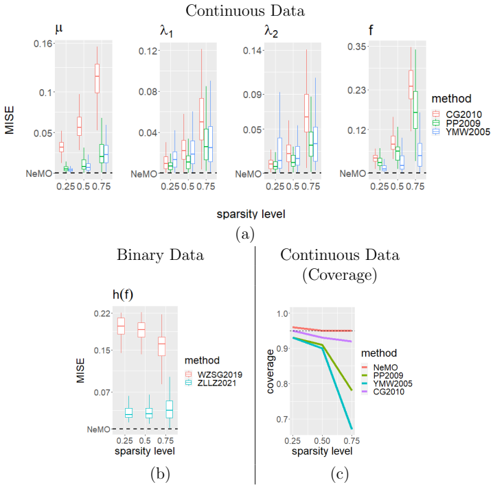
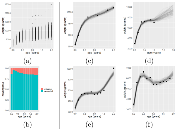
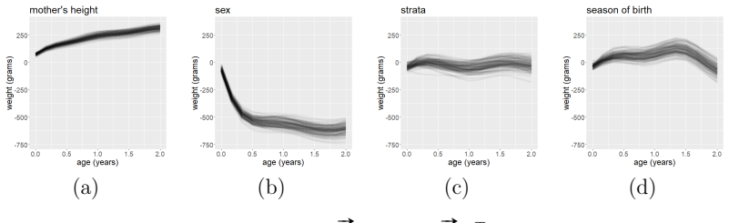
Functional factor analysis is an important dimension reduction method for functional and longitudinal data. Factor loadings give insight into patterns of variability of the observations, while latent factors provide a low-dimensional representation of the data that is useful for inferential tasks. Constraining the functional factor loadings to be mutually orthogonal is desirable for model parsimony but is computationally challenging. In this work, we introduce nearly mutually orthogonal processes, which can be used to effectively enforce mutual orthogonality of factor loadings while maintaining computational simplicity and efficiency. The joint distribution is governed by a penalty parameter that determines the degree to which the processes are mutually orthogonal and is related to ease of posterior computation. We demonstrate that our approach can be used for flexible and interpretable inference in an application to studying the effects of breastfeeding status, illness, and demographic factors on weight dynamics in early childhood. Code is available on GitHub: https://github.com/jamesmatuk/NeMO-FFA
Figures

Figures from the paper (25 more)










Lean theorems connected to this paper
-
IndisputableMonolith/Cost/FunctionalEquation.leanwashburn_uniqueness_aczel unclear?
unclearRelation between the paper passage and the cited Recognition theorem.
nearly mutually orthogonal processes... joint distribution governed by a penalty parameter νλ... exp(-1/(2νλ) ∑∑ ⟨λj,λk⟩²)
-
IndisputableMonolith/Foundation/RealityFromDistinction.leanreality_from_one_distinction unclear?
unclearRelation between the paper passage and the cited Recognition theorem.
Proposition 2.4... conditional covariance C^νλ_k(s,t) = Ck(s,t) - h... (νλ I + H)^{-1} h
What do these tags mean?
- matches
- The paper's claim is directly supported by a theorem in the formal canon.
- supports
- The theorem supports part of the paper's argument, but the paper may add assumptions or extra steps.
- extends
- The paper goes beyond the formal theorem; the theorem is a base layer rather than the whole result.
- uses
- The paper appears to rely on the theorem as machinery.
- contradicts
- The paper's claim conflicts with a theorem or certificate in the canon.
- unclear
- Pith found a possible connection, but the passage is too broad, indirect, or ambiguous to say the theorem truly supports the claim.
Forward citations
Cited by 2 Pith papers
-
Multi-output Orthogonal Gaussian Processes for Noisy Simulator Outputs
MOOGP extends orthogonal Gaussian processes to multi-output simulators, improving trend coefficient identifiability while retaining predictive accuracy.
-
Efficient Bayesian Inference for Discretely Observed Continuous Time Markov Chains
Bayesian inference for discretely observed CTMCs via a pseudo-likelihood that couples the transition matrix to a spectral generator, with a Gibbs sampler whose cost per iteration is near-invariant in the number of obs...
Reference graph
Works this paper leans on
-
[1]
M., VanDerslice, J., Akin, J., Guilkey, D., Black, R., Briscoe, J
Adair, L., Popkin, B. M., VanDerslice, J., Akin, J., Guilkey, D., Black, R., Briscoe, J. & Flieger, W. (1993), ‘Growth dynamics during the first two years of life: A prospective study in the Philippines’, European Journal of Clinical Nutrition 47(1), 42–51. Adair, L. S. & Guilkey, D. K. (1997), ‘Age-specific determinants of stunting in Filipino children’, T...
work page 1993
-
[2]
55 Jiang, L., Zhong, Y., Elrod, C., Natarajan, L., Knight, R. & Thompson, W. K. (2020), ‘Bayestime: Bayesian functional principal components for sparse longitudinal data’, arXiv:2012.00579. Khan, K. & Calder, C. A. (2022), ‘Restricted spatial regression methods: Implications for inference’, Journal of the American Statistical Association 117(537), 482–494...
-
[3]
URL: https://doi.org/10.1214/20-BA1213 Kowal, D. R. & Canale, A. (2021), ‘Semiparametric functional factor models with Bayesian rank selection’, arXiv:108.02151. Kowal, D. R., Matteson, D. S. & Ruppert, D. (2017), ‘A Gaussian multivariate functional dynamic linear model’, Journal of the American Statistical Association 112(518), 733–
-
[4]
Lenk, P. J. & Choi, T. (2017), ‘Bayesian analysis of shape-restricted functions using Gaus- sian process priors’, Statistica Sinica pp. 43–69. Lin, L. & Dunson, D. B. (2014), ‘Bayesian monotone regression using Gaussian process projection’, Biometrika 101(2), 303–317. Malfait, N. & Ramsay, J. O. (2003), ‘The historical functional linear model’, Canadian J...
-
[5]
Tipping, M. E. & Bishop, C. M. (1999), ‘Probabilistic principal component analysis’, Jour- nal of the Royal Statistical Society: Series B 61(3), 611–622. van der Linde, A. (2008), ‘Variational Bayesian functional PCA’, Computational Statistics & Data Analysis 53, 517–533. van der Linde, A. (2009), ‘A Bayesian latent variable approach to functional princip...
-
[6]
Children tend to experience cough more often than fever and fever more often than diarrhea
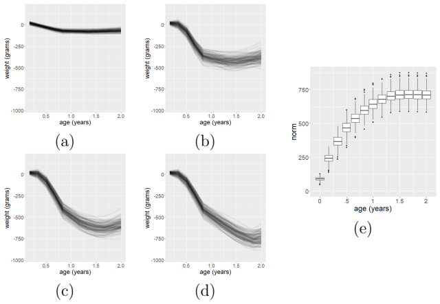
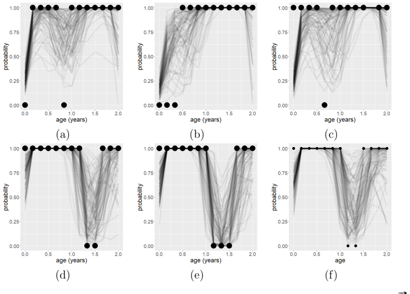
61 (a) (b) (c) (d) (e) (f) Figure 16: (a)-(c) Posterior samples of Φ(µzj( # »t )) for j = 2, 3, 4, representing the proportion of children in the study that experienced an illness by age.(d)-(f) Posterior samples ofβj( # »t ), j = 2 , 3, 4, representing the effect of experiencing an illness on weight. Children tend to experience cough more often than fever...
work page 2010
-
[7]
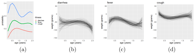
(f) Boxplots of posterior samples of ∥ ∫ T ˆβ11s≤s′ds∥2 for different values of s′. 63 (a) (b) (c) (d) Figure 19: Inferred functions related to modelling the effects of illness on weight using the Crainiceanu & Goldsmith (2010) model: (a) logit −1(ˆµzj(t)). (b)-(d) Posterior samples of βj(t) for j = 2, 3,
work page 2010
-
[8]
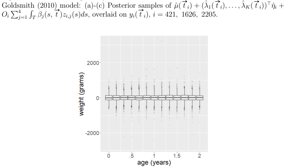
,ˆλK( # »t i))⊤ˆηi + Oi ∑4 j=1 ∫ T βj(s, # »t )zi,j(s)ds, overlaid on yi( # »t i), i = 421, 1626,
(a) (b) (c) Figure 20: Inferred weight trajectories for different subjects using the Crainiceanu & Goldsmith (2010) model: (a)-(c) Posterior samples of ˆ µ( # »t i) + (ˆλ1( # »t i), . . . ,ˆλK( # »t i))⊤ˆηi + Oi ∑4 j=1 ∫ T βj(s, # »t )zi,j(s)ds, overlaid on yi( # »t i), i = 421, 1626,
work page 2010
Reviewed May 24, 2026 · model on record in the stance chip above.
Discussion (0). Sign in to comment.