Nonlinear filtering based on density approximation and deep BSDE prediction
Pith reviewed 2026-05-18 23:13 UTC · model grok-4.3
The pith
A new approximate Bayesian filter uses nonlinear Feynman-Kac representation and deep BSDE to approximate the unnormalized filtering density with a hybrid error bound.
A machine-rendered reading of the paper's core claim, the machinery that carries it, and where it could break.
Core claim
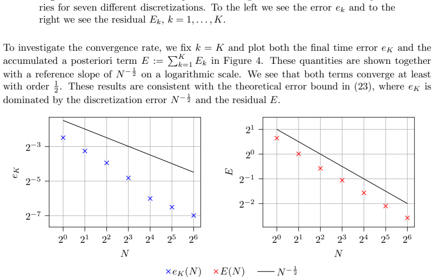
The paper establishes a novel approximate Bayesian filter that employs a nonlinear Feynman-Kac representation of the filtering problem together with the deep BSDE method and neural networks to approximate the unnormalized filtering density. The resulting scheme is trained offline and then applied online to new observations. Under the parabolic Hörmander condition a hybrid a priori-a posteriori error bound is proved, and the predicted convergence rate is verified numerically on two test problems.
What carries the argument
Nonlinear Feynman-Kac representation combined with deep BSDE approximation of the unnormalized filtering density; this representation converts the filtering density evolution into a backward stochastic differential equation that neural networks can solve offline.
Load-bearing premise
The underlying stochastic system must satisfy the parabolic Hörmander condition so that the hybrid error bound for the density approximation holds.
What would settle it
Run the method on a diffusion whose generator fails the parabolic Hörmander condition and check whether the observed approximation error still decays at the rate predicted by the hybrid bound.
Figures


read the original abstract
A novel approximate Bayesian filter based on backward stochastic differential equations is introduced. It uses a nonlinear Feynman--Kac representation of the filtering problem and the approximation of an unnormalized filtering density using the well-known deep BSDE method and neural networks. The method is trained offline, which means that it can be applied online with new observations. A hybrid a priori-a posteriori error bound is proved under a parabolic H\"ormander condition. The theoretical convergence rate is confirmed in two numerical examples.
Editorial analysis
A structured set of objections, weighed in public.
Referee Report
Summary. The paper introduces a novel approximate Bayesian filter that uses a nonlinear Feynman-Kac representation of the filtering problem and approximates the unnormalized filtering density via the deep BSDE method with neural networks. The approach is trained offline for online application with new observations. A hybrid a priori-a posteriori error bound is proved under a parabolic Hörmander condition, and the theoretical convergence rate is confirmed numerically in two examples.
Significance. If the hybrid error bound is valid and the numerical confirmation is robust, the work provides a theoretically supported method for nonlinear filtering that combines BSDE approximations with density estimation. This could be useful for high-dimensional problems. The offline training aspect is a practical advantage, and the hybrid bound represents a constructive attempt to blend a priori analysis with a posteriori control. The numerical examples offer some empirical support for the claimed rate.
major comments (2)
- [Abstract and theoretical analysis section] Abstract and theoretical analysis section: The hybrid a priori-a posteriori error bound is proved under the parabolic Hörmander condition to control the density approximation error inside the nonlinear Feynman-Kac representation. However, the manuscript provides no verification that the driving SDEs in the two numerical examples satisfy the Lie-algebra rank condition on the relevant time interval. This assumption is load-bearing for the claimed convergence rate, as its failure would collapse the a-priori component of the bound.
- [Section on deep BSDE approximation and error analysis] Section on deep BSDE approximation and error analysis: The paper does not demonstrate that the neural-network error from the deep BSDE training step inherits the hypoelliptic regularity supplied by the parabolic Hörmander condition. Without this link, it is unclear whether the practical algorithm inherits the theoretical rate, even if the underlying SDE satisfies the assumption.
minor comments (2)
- [Method section] The definition of the unnormalized filtering density and its relation to the nonlinear Feynman-Kac representation could be stated more explicitly at the beginning of the method section for improved readability.
- [Numerical examples] Numerical example figures would benefit from additional details in the captions regarding the specific parameters, time horizons, and network architectures used to confirm the convergence rate.
Simulated Author's Rebuttal
We thank the referee for their careful reading of the manuscript and for the constructive major comments. We address each point below and indicate the revisions that will be incorporated in the next version.
read point-by-point responses
-
Referee: [Abstract and theoretical analysis section] Abstract and theoretical analysis section: The hybrid a priori-a posteriori error bound is proved under the parabolic Hörmander condition to control the density approximation error inside the nonlinear Feynman-Kac representation. However, the manuscript provides no verification that the driving SDEs in the two numerical examples satisfy the Lie-algebra rank condition on the relevant time interval. This assumption is load-bearing for the claimed convergence rate, as its failure would collapse the a-priori component of the bound.
Authors: We agree that an explicit verification of the Lie-algebra rank condition for the driving SDEs in the numerical examples strengthens the link between theory and experiments. Both examples were selected from the standard nonlinear filtering literature precisely because they satisfy the parabolic Hörmander condition on the intervals considered; the first is uniformly elliptic and the second has a diffusion coefficient whose Lie brackets span the tangent space. In the revised manuscript we will add a short paragraph (or subsection) that recalls the relevant vector fields and confirms the rank condition holds, thereby making the applicability of the hybrid bound fully transparent. revision: yes
-
Referee: [Section on deep BSDE approximation and error analysis] Section on deep BSDE approximation and error analysis: The paper does not demonstrate that the neural-network error from the deep BSDE training step inherits the hypoelliptic regularity supplied by the parabolic Hörmander condition. Without this link, it is unclear whether the practical algorithm inherits the theoretical rate, even if the underlying SDE satisfies the assumption.
Authors: The hybrid bound separates the error into an a-priori term that exploits the hypoelliptic regularity to control the density approximation inside the nonlinear Feynman-Kac representation and an a-posteriori term that controls the deep-BSDE neural-network training error via standard empirical-risk bounds. The regularity guarantees that the associated PDE solution is sufficiently smooth for the BSDE to be well-defined and for the neural-network approximation theory to apply with the expected rate. To make this inheritance explicit we will insert a clarifying remark in the error-analysis section that recalls how hypoelliptic regularity propagates to the BSDE solution and thereby justifies the use of the same convergence rate for the neural-network component. This addition will remove any ambiguity about whether the practical algorithm inherits the theoretical rate. revision: partial
Circularity Check
No significant circularity; derivation relies on external Hörmander condition and standard deep BSDE
full rationale
The paper's central derivation introduces a nonlinear Feynman-Kac representation of the filtering problem, approximates the unnormalized density via the established deep BSDE method with neural networks, and proves a hybrid a priori-a posteriori error bound under the parabolic Hörmander condition. This condition is a standard external assumption from stochastic analysis (hypoelliptic regularity) rather than a self-derived or self-cited result. The deep BSDE training is offline and uses well-known techniques without any fitted parameters being renamed as predictions or any self-definitional loops in the equations. Numerical examples confirm rates but do not constitute the theoretical claim. No load-bearing step reduces by construction to the paper's own inputs; the argument remains self-contained against external benchmarks.
Axiom & Free-Parameter Ledger
free parameters (1)
- Neural network weights and biases
axioms (1)
- domain assumption Parabolic Hörmander condition on the diffusion coefficients
Lean theorems connected to this paper
-
IndisputableMonolith/Foundation/AlexanderDuality.leanalexander_duality_circle_linking unclear?
unclearRelation between the paper passage and the cited Recognition theorem.
A hybrid a priori-a posteriori error bound is proved under a parabolic Hörmander condition... span{Vj1(x), [Vj1,Vj2], ...} = Rd (3)
-
IndisputableMonolith/Cost/FunctionalEquation.leanwashburn_uniqueness_aczel unclear?
unclearRelation between the paper passage and the cited Recognition theorem.
deep BSDE method... optimization problem (15)... Theorem 3.1 mixed a priori and a posteriori bound
What do these tags mean?
- matches
- The paper's claim is directly supported by a theorem in the formal canon.
- supports
- The theorem supports part of the paper's argument, but the paper may add assumptions or extra steps.
- extends
- The paper goes beyond the formal theorem; the theorem is a base layer rather than the whole result.
- uses
- The paper appears to rely on the theorem as machinery.
- contradicts
- The paper's claim conflicts with a theorem or certificate in the canon.
- unclear
- Pith found a possible connection, but the passage is too broad, indirect, or ambiguous to say the theorem truly supports the claim.
Forward citations
Cited by 1 Pith paper
-
High-dimensional Bayesian filtering through deep density approximation
The logarithmic deep backward SDE filter succeeds in a 100-dimensional Lorenz-96 model where particle and ensemble Kalman filters fail, while cutting inference time by two to five orders of magnitude.
Reference graph
Works this paper leans on
-
[1]
K. Andersson, A. Andersson, and C. W. Oosterlee. The deep multi-FBSDE method: a robust deep learning method for coupled FBSDEs. arXiv:2503.13193, 2025
-
[2]
K. B˚ agmark, A. Andersson, and S. Larsson. An energy-based deep splitting method for the nonlinear filtering problem. Partial Differ. Equ. Appl. , 4, 2023
work page 2023
-
[3]
K. B˚ agmark, A. Andersson, S. Larsson, and F. Rydin. A convergent scheme for the Bayesian filtering problem based on the Fokker–Planck equation and deep splitting. arXiv:2409.14585, 2024
work page internal anchor Pith review Pith/arXiv arXiv 2024
-
[4]
Y. Bar-Shalom, X. R. Li, and T. Kirubarajan. Estimation with Applications to Tracking and Navigation . John Wiley & Sons, 2001
work page 2001
-
[5]
C. Beck, S. Becker, P. Cheridito, A. Jentzen, and A. Neufeld. Deep learning based numerical approxima- tion algorithms for stochastic partial differential equations and high-dimensional nonlinear filtering problems. arXiv:2012.01194, 2020. NONLINEAR FILTERING BASED ON DENSITY APPROXIMATION AND DEEP BSDE PREDICTION 17
-
[6]
C. Beck, S. Becker, P. Cheridito, A. Jentzen, and A. Neufeld. Deep splitting method for parabolic PDEs. SIAM J. Sci. Comput. , 43:A3135–A3154, 2021
work page 2021
-
[7]
S. S. Blackman and R. Popoli. Design and Analysis of Modern Tracking Systems . Artech House Publishers, 1999
work page 1999
-
[8]
S. Challa and Y. Bar-Shalom. Nonlinear filter design using Fokker-Planck-Kolmogorov probability density evolutions. IEEE Trans. Aerosp. Electron. Syst., 36:309–315, 2000
work page 2000
- [9]
-
[10]
A. Corenflos and A. Finke. Particle-MALA and Particle-mGRAD: Gradient-based MCMC methods for high- dimensional state-space models. arXiv:2401.14868, 2024
-
[11]
A. Corenflos, Z. Zhao, T. B. Sch¨ on, S. S¨ arkk¨ a, and J. Sj¨ olund. Conditioning diffusion models by explicit forward-backward bridging. In Int. Conf. Artif. Intell. Stat. , pages 3709–3717. PMLR, 2025
work page 2025
- [12]
-
[13]
N. Cui, L. Hong, and J. R. Layne. A comparison of nonlinear filtering approaches with an application to ground target tracking. Signal Processing, 85:1469–1492, 2005
work page 2005
-
[14]
B. Demissie, M. A. Khan, and F. Govaers. Nonlinear filter design using Fokker-Planck propagator in Kronecker tensor format. In 2016 19th International Conference on Information Fusion (FUSION) , pages 1–8. IEEE, 2016
work page 2016
-
[15]
W. E, J. Han, and A. Jentzen. Deep learning-based numerical methods for high-dimensional parabolic partial differential equations and backward stochastic differential equations. Commun. Math. Stat , 5:349–380, Nov. 2017
work page 2017
-
[16]
W. E and B. Yu. The deep Ritz method: A deep learning-based numerical algorithm for solving variational problems. Commun. Math. Stat , 1:1–12, 2018
work page 2018
-
[17]
N. El Karoui, S. Peng, and M. C. Quenez. Backward stochastic differential equations in finance. Math. Finance, 7(1):1–71, 1997
work page 1997
-
[18]
G. Evensen. Data Assimilation: The Ensemble Kalman Filter . Springer, 2009
work page 2009
-
[19]
A. Finke and A. H. Thiery. Conditional sequential Monte Carlo in high dimensions. Ann. Statist., 51:437–463, 2023
work page 2023
-
[20]
M. B. Giles. Multilevel Monte Carlo methods. Acta Numerica, 24:259–328, 2015
work page 2015
-
[21]
I. R. Goodman, R. P. S. Mahler, and H. T. Nguyen. Mathematics of Data Fusion , volume 37 of Theory and Decision Library. Series B: Mathematical and Statistical Methods . Kluwer Academic Publishers Group, Dordrecht, 1997
work page 1997
-
[22]
N. J. Gordon, D. J. Salmond, and A. F. M. Smith. Novel approach to nonlinear/non-Gaussian Bayesian state estimation. IEE Proceedings F (Radar and Signal Processing) , 140(2):107–113, 1993
work page 1993
-
[23]
F. K. Gustafsson, M. Danelljan, G. Bhat, and T. B. Sch¨ on. Energy-based models for deep probabilistic regres- sion. In European Conference on Computer Vision , pages 325–343. Springer, 2020
work page 2020
- [24]
- [25]
- [26]
-
[27]
J. Ho, A. Jain, and P. Abbeel. Denoising diffusion probabilistic models.Adv. Neural Inf. Process. Syst., 33:6840– 6851, 2020
work page 2020
-
[28]
M. Isard and A. Blake. Condensation—conditional density propagation for visual tracking. Int. J. Comput. Vis., 29(1):5–28, 1998
work page 1998
- [29]
-
[30]
M. S. Johannes and N. G. Polson. MCMC Methods for Continuous-Time Financial Econometrics. In Handbook of Financial Econometrics , pages 1–72. Elsevier, 2009
work page 2009
-
[31]
R. E. Kalman and R. S. Bucy. New results in linear filtering and prediction theory. J. Basic Eng. , 83:95–108, 1961
work page 1961
-
[32]
L. Kapllani and L. Teng. A backward differential deep learning-based algorithm for solving high-dimensional nonlinear backward stochastic differential equations. IMA J. Numer. Anal. , 2025
work page 2025
-
[33]
K. P. K¨ ording and D. M. Wolpert. Bayesian integration in sensorimotor learning. Nature, 427(6971):244–247, 2004
work page 2004
-
[34]
A. Krishnapriyan, A. Gholami, S. Zhe, R. Kirby, and M. W. Mahoney. Characterizing possible failure modes in physics-informed neural networks. Adv. Neural Inf. Process. Syst. , 34:26548–26560, 2021
work page 2021
-
[35]
L. Lu, P. Jin, G. Pang, Z. Zhang, and G. E. Karniadakis. Learning nonlinear operators via DeepONet based on the universal approximation theorem of operators. Nat. Mach. Intell. , 3:218–229, 2021
work page 2021
-
[36]
K. Luo, J. Zhao, Y. Wang, J. Li, J. Wen, J. Liang, H. Soekmadji, and S. Liao. Physics-informed neural networks for PDE problems: a comprehensive review. Artif. Intell. Rev. , 58(10):1–43, 2025
work page 2025
-
[37]
P. S. Maybeck. Stochastic Models, Estimation, and Control, Volume 1 . Academic Press, 1979
work page 1979
-
[38]
C. A. Naesseth, F. Lindsten, and T. B. Sch¨ on. High-dimensional filtering using nested sequential Monte Carlo. IEEE Trans. Signal Process., 67:4177–4188, 2019. 18 K. B ˚AGMARK, A. ANDERSSON, AND S. LARSSON
work page 2019
- [39]
- [40]
-
[41]
R. Rombach, A. Blattmann, D. Lorenz, P. Esser, and B. Ommer. High-resolution image synthesis with latent diffusion models. In Proc. IEEE/CVF Conf. Comput. Vis. Pattern Recognit. , pages 10684–10695, 2022
work page 2022
-
[42]
O. Ronneberger, P. Fischer, and T. Brox. U-Net: Convolutional Networks for Biomedical Image Segmentation. In Med. Image Comput. Comput. Assist. Interv. , pages 234–241. Springer, 2015
work page 2015
- [43]
-
[44]
C. Snyder. Particle filters, the “optimal” proposal and high-dimensional systems. In Proceedings of the ECMWF Seminar on Data Assimilation for atmosphere and ocean , pages 1–10, 2011
work page 2011
- [45]
-
[46]
Y. Song, J. Sohl-Dickstein, D. P. Kingma, A. Kumar, S. Ermon, and B. Poole. Score-based generative modeling through stochastic differential equations. In Int. Conf. Learn. Represent., 2021
work page 2021
- [47]
-
[48]
F. van der Meulen and M. Schauer. Automatic backward filtering forward guiding for Markov processes and graphical models. arXiv:2010.03509, 2020
-
[49]
A. Vaswani, N. Shazeer, N. Parmar, J. Uszkoreit, L. Jones, A. N. Gomez, L. Kaiser, and I. Polosukhin. Attention is all you need. Adv. Neural Inf. Process. Syst. , 30:5998–6008, 2017
work page 2017
-
[50]
Z. Zhao, Z. Luo, J. Sj¨ olund, and T. B. Sch¨ on. Conditional sampling within generative diffusion models. arXiv:2409.09650, 2024. Appendix A. Implementation details A.1. Networks and training. The spaces NNΘ,p, p = 1 or p = d, where we define our models consist of fully connected feed-forward neural networks with three hidden layers, one input layer, and...
discussion (0)
Sign in with ORCID, Apple, or X to comment. Anyone can read and Pith papers without signing in.