REVIEW 3 major objections 5 minor 1 cited by
Numerical Study of Random Kelvin-Helmholtz Instability
T0 review · 3 major / 5 minor · reviewed 2026-08-04 · deepseek-v4-flash
Pith's one-line read Random Kelvin–Helmholtz instabilities in compressible Euler flow have reproducible statistical structure even though individual solutions do not.
desk verdict Useful numerical observations, but the 'random' in the title is really a one-parameter family; the paper deserves review once the authors close the gap between the sampling and the claim. read the letter →
The pith
A machine-rendered reading of the paper's core claim, the machinery that carries it, and where it could break.
The reading
What carries the argument
The central objects are random dissipative weak (DW) solutions: defect-modified weak solutions of the Euler equations in which unresolved oscillations are encoded by Reynolds stress and energy defect rather than by a single pointwise solution. The machinery is stochastic collocation in a one-dimensional random space (uniform collocation points, CWENO7 interpolation, exact integration for the uniform measure), embedded uniform meshes whose solutions are combined into Cesàro averages, and defect formulas that turn averaged moments into turbulence diagnostics. Theorems 2.1 and 2.2 assert strong convergence of Cesàro and Monte-Carlo averages to this DW solution, which is what licenses interpreti
What would settle it
Compute the same statistical setup with far more than 101 collocation points, with multi-dimensional random inputs, or with more than five embedded meshes, and check whether the Reynolds-stress and energy defects continue to decrease. If the defects stop converging or POD mode counts keep growing with resolution, the claimed saturation and stabilization are false. A sharper test: run the same flow with the Navier–Stokes equations at progressively smaller viscosity and compare the averaged defect measures to those predicted here; a mismatch would show that the DW statistical description does no
Extended reading notes
Core claim
On the paper's own terms, the discovery is that a randomized Kelvin–Helmholtz instability can be meaningfully characterized by averaged quantities. Random interface perturbations (controlled by a scalar ξ and ten random Fourier coefficients per interface) are propagated with a fifth-order A-WENO scheme on five embedded meshes; solutions are interpolated in random space with seventh-order CWENO and averaged to Cesàro means. The Reynolds-stress and energy defects computed from these averages satisfy the theoretical bounds of dissipative weak solutions, converge as the mesh index increases, and the ratio of energy to stress defects approaches the predicted slope. The POD analysis shows that the
Load-bearing premise
The central load-bearing premise is that the Cesàro and Monte-Carlo averages converge to a random dissipative weak solution—a convergence asserted by analogy to a related barotropic result but not proved here—together with the practical assumption that one scalar random variable and five embedded meshes capture the essential randomness of the instability.
Editorial extensions
If this is right
- Cesàro-averaged solutions on five embedded meshes approximate a random DW solution, so averaged fields can be used where deterministic weak solutions are non-unique.
- Reynolds stress and energy defects, the unresolved-fluctuation signatures, shrink consistently with mesh index and their ratio stays within the theoretical bounds, making them usable as quantitative statistical monitors.
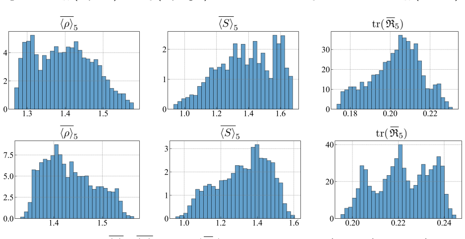
- PDFs of averaged density, entropy, and stress in fixed spatial windows have non-Dirac support, indicating genuine stochastic variability rather than convergence to a single realization.
- POD mode counts saturate around 76–78 modes for fine meshes across all perturbation strengths, implying a bounded reduced-order complexity for these flows; coarser meshes need only 20–50 modes.
- Cesàro averaging reduces the effective dimensionality, with fewer POD modes for averaged density than for raw density, so statistical averaging acts as a practical compression strategy for chaotic flow data.
Reading between the lines
- A natural next test is to replace the single scalar random variable with a genuinely multi-dimensional random input; if the reported statistics change qualitatively, the present results describe only a narrow slice of the randomness.
- The saturation of POD mode counts near 80 suggests an intrinsic stochastic attractor dimension for this configuration; if it persists at even finer meshes, it points to a resolution-independent reduced-order model.
- One could connect the observed energy and Reynolds defects to the viscous dissipation of an underlying Navier–Stokes flow: at small but finite viscosity, the defect measures should match turbulent dissipation rates, tying the DW framework to physical turbulence modeling.
- The unproved Theorem 2.2 is the bridge between the numerical averages and the DW solution concept; until it is supplied, the statistical claims rest on numerical evidence rather than a fully established convergence result.
Editorial analysis
A structured set of objections, weighed in public.
Referee Report
Summary. The paper proposes a numerical framework for studying random dissipative weak (DW) solutions of the compressible Euler equations, applied to the Kelvin–Helmholtz instability. The method combines A-WENO spatial discretizations on embedded uniform meshes with stochastic collocation in a one-dimensional random variable ξ, forms Cesàro averages over M=5 meshes, and computes diagnostics: Reynolds stress and energy defects, PDFs of averaged quantities, and POD mode counts. The authors claim that these tools reveal turbulence-like statistical structure and that random KH instabilities can be meaningfully characterized by a turbulence-inspired statistical framework. The theoretical justification relies on Theorem 2.2, which is asserted but not proved.
Significance. If the central claim were fully supported, the paper would provide a practical way to extract well-behaved observables from an ill-posed inviscid problem: defect residuals decrease with M (Fig. 4.6), defect ratios remain within the theoretical bounds of (2.2), and POD mode counts appear to saturate around 76–78 for the finest mesh, suggesting a moderate-dimensional reduced basis. The numerical pipeline is clearly described and reproducible in principle, and the diagnostics are internally consistent. However, the stochastic representation used in the experiments is too narrow to support the paper's broad claim about random KH instabilities, and the theoretical basis for interpreting the computed means is not made rigorous.
major comments (3)
- [§3, Eq. (4.2)] The stochastic dimension is reduced to s=1 by fixing the random coefficients a_i^k, b_i^k after a single draw ('generated once for repeatability') and treating ξ as the only random variable. Thus the ensemble averages, PDFs, defects, and POD results in Figures 4.4–4.9 and Tables 4.1–4.4 are conditional on one realization of the 20 Fourier phases/amplitudes. A different draw changes the spatial structure of the shear-layer perturbation, not just its amplitude. No sensitivity analysis or argument that the single draw is representative is provided. This directly undermines the §5 conclusion that 'random KH instabilities can be meaningfully characterized using a turbulence-inspired statistical framework.' The authors should either sample a_i^k, b_i^k (e.g., by stochastic collocation or Monte Carlo in the full 21-dimensional space) or explicitly restrict the claim to the one-dimensional famil
- [§2.2, Theorem 2.2] Theorem 2.2 is asserted without proof; the manuscript says only that its proof can be established analogously to [14, Theorem 5.6] for the barotropic system. This theorem is the theoretical basis for interpreting the computed means of Cesàro averages as approximations of the expected DW solution. In addition, the theorem is formulated for Monte Carlo averages over i.i.d. samples (indexed by ℓ), whereas the numerical method uses deterministic collocation points in ξ with a high-order interpolation/quadrature. No argument is given that the collocation means converge to the same limit as the Monte Carlo means. The authors should provide a proof or a precise citation covering the collocation case, or soften the theoretical framing of §4.
- [Tables 4.1–4.4] The POD analysis uses L=101 collocation snapshots for each mesh m, so the data matrix has rank at most 101. The claimed 'saturating' mode count of 76–78 at m=5 could be influenced by the fixed finite snapshot count; no study of the dependence on L is reported. A convergence check in L (e.g., L=51, 101, 201) is needed before concluding that the mode count saturates as a property of the flow rather than as an artifact of the snapshot set.
minor comments (5)
- [Appendix A, Eq. (A.2)] In the momentum identity, the first term should be m·∂_t φ, not m·φ. As printed, the variational formulation is missing the time derivative.
- [§2.2, Theorem 2.2] The target space is written as L^q(T^d×(0,T); R^{d+1}); for the state (ρ,m,S) this should be R^{d+2}, matching Theorem 2.1.
- [§4, Figure 4.5] The text says the ratio E5/tr(R5) stays within the 'theoretically bounds 0.5 and 1.25, specified in (2.2).' These are actually the inverse bounds 1/d2 and 1/d1 for d=2 and the chosen γ. Please clarify that the plotted ratio is E/trR and relate it explicitly to (2.2).
- [§3, Eq. (3.5)] The definition of R_M and E_M does not make clear whether the expectation over ξ (as in (3.2)) is applied inside the defect formulas or whether the displayed quantities are pointwise in ξ. Please define explicitly, e.g., R_M(x,y) = E[ ... ] or R_M(x,y;ξ).
- [§4.1.1] The singular value decay in Figure 4.9 is shown for m=1 and m=5 only; the caption and text would benefit from specifying the mesh sizes N_m used.
Circularity Check
No circularity: the reported statistical quantities are diagnostics computed from simulated data, not fitted parameters or inputs renamed as predictions.
full rationale
The paper's central quantities — Cesàro averages (2.3), Reynolds stress/energy defects (3.5), PDFs (3.4), and POD mode counts (Tables 4.1–4.4) — are computed from the numerical solutions rather than imposed. Equation (3.5) is a definition used to post-process the averages; the convergence of ϵ_R and ϵ_E in Figure 4.6 is a numerical observation and is not forced by construction, since tr(R_M) is a nonlinear function of the partial Cesàro average, not an average of the per-mesh defects. The POD analysis performs an SVD of snapshot matrices and reports cumulative energy; no parameter is fitted to the final statistics. Therefore no step makes a 'prediction' equivalent to an input. The main caveats are non-circular: Theorem 2.2 is stated without proof ('Its proof can be established analogously to the proof of [14, Theorem 5.6]'), deferring to a preprint with overlapping authors and a different (barotropic) system; and the stochastic space is reduced to s=1 in §3 while the random coefficients a_i^k, b_i^k in Eq. (4.2) are drawn once, so the reported expectations are conditional on that single draw. These gaps limit the force of the general 'random KH' claim, but they are missing-support/correctness concerns, not reductions of outputs to inputs.
Assumptions & free parameters
free parameters (7)
- τ (interface perturbation amplitude) =
1.1 (default; varied in [0,1.1])
- M (number of embedded grids) =
5
- L (number of collocation points in ξ) =
101
- T (final time) =
2
- m0 (mesh-level offset) =
unspecified
- Spatial windows D1, D2 =
D1=[0.46,0.54]×[0.71,0.79], D2=[0.76,0.84]×[0.71,0.79]
- Number of Fourier harmonics K =
10
assumptions (6)
- domain assumption The compressible Euler system admits infinitely many weak entropy solutions, and the dissipative weak solution framework from [11] is the appropriate selection criterion.
- standard math Theorem 2.1 (K-convergence of Cesàro averages) and the weak-strong uniqueness/compatibility properties hold as stated in [13] and [11].
- ad hoc to paper Theorem 2.2: Monte Carlo/Cesàro averages of consistent stable approximations converge strongly to a random dissipative weak solution for the full compressible Euler system.
- domain assumption Numerical solutions produced by the fifth-order A-WENO scheme [6] are consistent and stable approximations in the sense required by Theorems 2.1–2.2.
- ad hoc to paper A single scalar random variable ξ entering only via tanh(ξ) in Eq. (4.2), with fixed random coefficients a_i^k, b_i^k, adequately represents random KH instabilities.
- domain assumption The CWENO7 piecewise polynomial interpolant (3.3) provides sufficiently accurate quadrature for computing moments (3.4).
Cite this review
Pith. "Pith review of Numerical Study of Random Kelvin-Helmholtz Instability." pith.science (2026). https://pith.science/paper/JPTNODTL
@misc{pith2026251100008,
  author       = {Pith},
  title        = {Pith review of: Numerical Study of Random Kelvin-Helmholtz Instability},
  year         = {2026},
  howpublished = {\url{https://pith.science/paper/JPTNODTL}},
  note         = {Machine review of arXiv:2511.00008}
}
read the original abstract
In this paper, we study random dissipative weak solutions of the compressible Euler equations in the Kelvin-Helmholtz (KH) instability. Motivated by the fact that weak entropy solutions are not unique and can be viewed as inviscid limits of Navier-Stokes flows, we take a statistical approach following ideas from turbulence theory. Our aim is to identify solution features that remain consistent across different realizations and mesh resolutions. For this purpose, we compute stable numerical solutions using a stochastic collocation method implemented with the help of a fifth-order alternative weighted essentially non-oscillatory (A-WENO) scheme and seventh-order central weighted essentially non-oscillatory (CWENO) interpolation in the random space. The obtained solutions are averaged over several embedded uniform grids, resulting in Ces\'aro averages, which are studied using stochastic tools. The analysis includes Reynolds stress and energy defects, probability density functions of averaged quantities, and reduced-order representations using proper orthogonal decomposition. The presented numerical experiments illustrate that random KH instabilities can be systematically described using statistical methods, averaging, and reduced-order modeling, providing a robust methodology for capturing the complex and chaotic dynamics of inviscid compressible flows.
Figures


Figures from the paper (6 more)




Forward citations
Cited by 1 Pith paper
-
Numerical Study of Dissipative Weak Solutions for the Euler Equations of Gas Dynamics
Different high-order numerical schemes for the compressible Euler equations yield different scheme-dependent dissipative weak solutions in oscillatory regimes, while order-averaged and time-averaged statistics look mo...
Reference graph
Works this paper leans on
-
[1]
Berkooz, P
G. Berkooz, P. Holmes, and J. L. Lumley , The proper orthogonal decomposition in the analysis of turbulent flows, in Annual review of fluid mechanics, V ol. 25, Annual Reviews, Palo Alto, CA, 1993, pp. 539--575
1993
-
[2]
B r ezina and E
J. B r ezina and E. Feireisl , Measure-valued solutions to the complete E uler system, J. Math. Soc. Japan, 70 (2018), pp. 1227--1245
2018
-
[3]
Chertock, S
A. Chertock, S. Chu, M. Herty, A. Kurganov, and M. Luk\' a c ov\' a -Medvi ov\' a , Local characteristic decomposition based central-upwind scheme, J. Comput. Phys., 473 (2023). Paper No. 111718
2023
-
[4]
Chertock, A
A. Chertock, A. S. Iskhakov, and A. Kurganov , Uncertainty quantification in forward problems: B alancing accuracy and robustness using CWENO interpolations. Submitted
-
[5]
Chiodaroli, C
E. Chiodaroli, C. De Lellis, and O. Kreml , Global ill-posedness of the isentropic system of gas dynamics, Comm. Pure Appl. Math., 68 (2015), pp. 1157--1190
2015
-
[6]
S. Chu, A. Kurganov, and R. Xin , A fifth-order A - WENO scheme based on the low-dissipation central-upwind fluxes, in Hyperbolic problems: theory, numerics, applications. V ol. II , vol. 35 of SEMA SIMAI Springer Ser., Springer, Cham, [2024] 2024, pp. 51--61
2024
-
[7]
Cravero, G
I. Cravero, G. Puppo, M. Semplice, and G. Visconti , C WENO : uniformly accurate reconstructions for balance laws, Math. Comp., 87 (2018), pp. 1689--1719
2018
-
[8]
De Lellis and L
C. De Lellis and L. Sz\' e kelyhidi, Jr. , On admissibility criteria for weak solutions of the E uler equations, Arch. Ration. Mech. Anal., 195 (2010), pp. 225--260
2010
Show all 21 references
-
[9]
Dumbser, O
M. Dumbser, O. Zanotti, and G. Puppo , Monolithic first-order BSSNOK formulation of the E instein- E uler equations and its solution with path-conservative finite difference central WENO schemes, Phys. Rev. D, 111 (2025). Paper No. 104072
2025
-
[10]
Feireisl, C
E. Feireisl, C. Klingenberg, and S. Markfelder , On the density of ``wild'' initial data for the compressible E uler system, Calc. Var. Partial Differential Equations, 59 (2020). Paper No. 152
2020
-
[11]
Feireisl, M
E. Feireisl, M. Luk\' a c ov\' a -Medvid'ov\' a , H. Mizerov\' a , and B. She , Numerical analysis of compressible fluid flows, vol. 20 of MS&A. Modeling, Simulation and Applications, Springer, Cham, 2021
2021
-
[12]
Feireisl, M
E. Feireisl, M. Luk\' a c ov\' a -Medvid'ov\' a , S. Schneider, and B. She , Approximating viscosity solutions of the E uler system, Math. Comp., 91 (2022), pp. 2129--2164
2022
-
[13]
Feireisl, M
E. Feireisl, M. Luk\' a c ov\' a -Medvid'ov\' a , B. She, and Y. Wang , Computing oscillatory solutions of the E uler system via K -convergence, Math. Models Methods Appl. Sci., 31 (2021), pp. 537--576
2021
-
[14]
Feireisl, M
E. Feireisl, M. Luk\' a c ov\' a -Medvi ov\' a , H. Mizerov\' a , and C. Yu , Monte C arlo method and the random isentropic E uler system, arXiv preprint arXiv:2404.11983, (2024)
2024 arXiv
-
[15]
U. S. Fjordholm, S. Mishra, and E. Tadmor , On the computation of measure-valued solutions, Acta Numer., 25 (2016), pp. 567--679
2016
-
[16]
Holmes, J
P. Holmes, J. L. Lumley, G. Berkooz, and C. W. Rowley , Turbulence, coherent structures, dynamical systems and symmetry, Cambridge Monographs on Mechanics, Cambridge University Press, Cambridge, second ed., 2012
2012
-
[17]
A. S. Monin and A. M. Yaglom , Statistical fluid mechanics: mechanics of turbulence. V ol. II , Dover Publications, Inc., Mineola, NY, 2007. Translated from the 1965 Russian original, Edited and with a preface by John L. Lumley, English edition updated, augmented and revised b...
2007
-
[18]
S. B. Pope , Turbulent flows, Cambridge University Press, Cambridge, 2000
2000
-
[19]
Xiu , Fast numerical methods for stochastic computations: a review, Commun
D. Xiu , Fast numerical methods for stochastic computations: a review, Commun. Comput. Phys., 5 (2009), pp. 242--272
2009
-
[20]
Xiu , Numerical methods for stochastic computations, Princeton University Press, Princeton, NJ, 2010
D. Xiu , Numerical methods for stochastic computations, Princeton University Press, Princeton, NJ, 2010. A spectral method approach
2010
-
[21]
write newline
" write newline "" before.all 'output.state := FUNCTION fin.entry add.period write newline FUNCTION new.block output.state before.all = 'skip after.block 'output.state := if FUNCTION not #0 #1 if FUNCTION and 'skip pop #0 if FUNCTION or pop #1 'skip if FUNCTION new.block.check...
Reviewed August 4, 2026 · model on record in the stance chip above.
Discussion (0). Continue with ORCID to comment.