REVIEW 5 major objections 7 minor 33 references
Deep Learning for Sea Surface Temperature Reconstruction under Cloud Occlusion
T0 review · 5 major / 7 minor · reviewed 2026-08-11 · deepseek-v4-flash
Pith's one-line read The paper claims that a U-Net trained on four nights of MODIS Aqua SST, with a seasonal climatology subtracted, fills cloud-occluded pixels with roughly half the root-mean-square error of established interpolation products.
desk verdict Solid engineering with reproducible code, but the headline 50% improvement claim is not supported by the paper's own comparisons, and the evaluation protocol has load-bearing flaws. read the letter →
The pith
A machine-rendered reading of the paper's core claim, the machinery that carries it, and where it could break.
The reading
What carries the argument
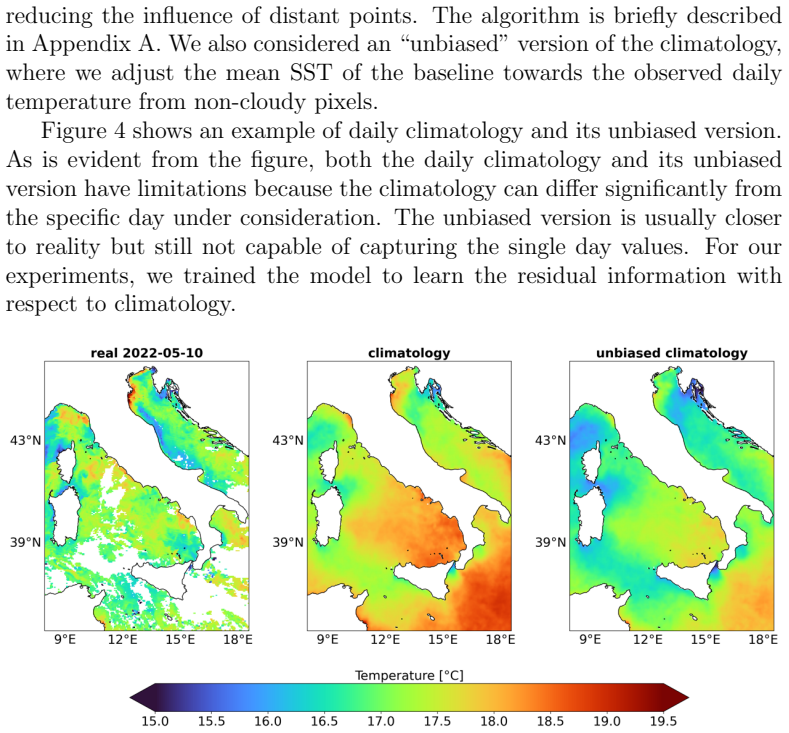
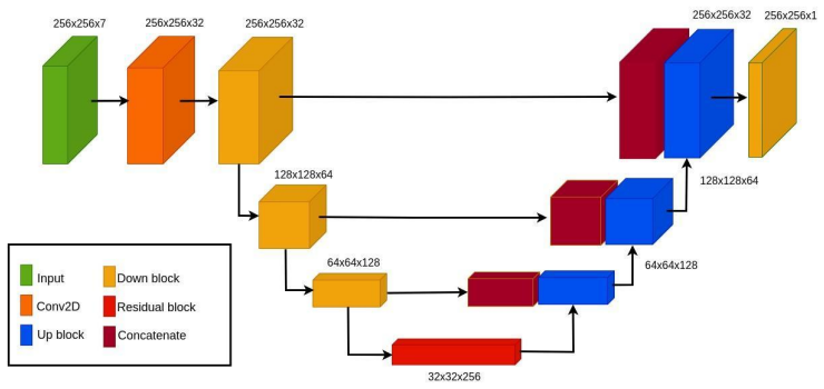
The load-bearing object is a U-Net with residual down- and up-sampling blocks and skip connections, configured as U-Net64 with channel structure [64,128,256,512], fed a temporal stack of the current night and four previous nights, each with its cloud mask, plus a land-sea mask. The target is the anomaly relative to an unbiased daily climatology, built by Gaussian-blur interpolation and temporal smoothing, so the network learns residual deviations rather than absolute temperatures. Training and evaluation rely on an artificial cloud generator that copies real cloud masks from other days onto clear-sky scenes, guaranteeing a controlled visible-sea fraction and defining the region where RMSE is measured. The same generator and the DINCAE baselines anchor the comparison.
What would settle it
Evaluate the U-Net64 reconstruction on real cloud-covered pixels using independent nighttime microwave SST retrievals or drifting-buoy measurements that see through clouds; if the RMSE advantage over L4 and DINCAE shrinks or reverses on those points, the central claim fails.
Extended reading notes
Core claim
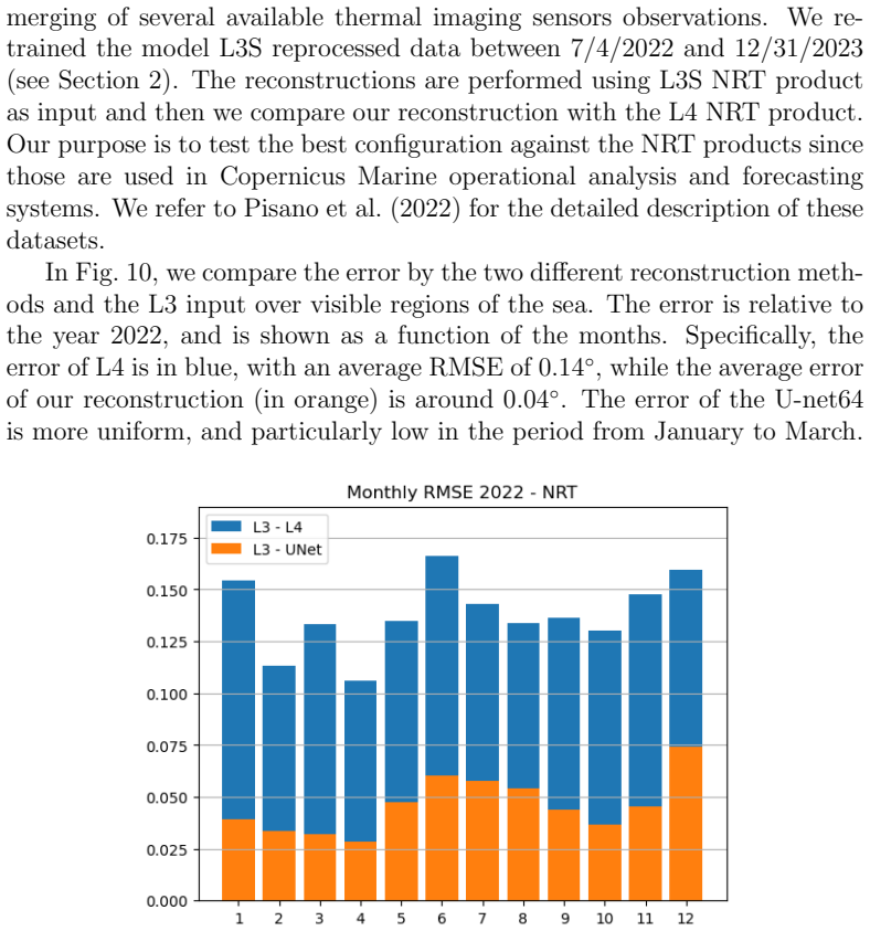
The central discovery is that a moderately sized U-Net, trained with a configurable artificial cloud generator on a residual anomaly target, outperforms both OI-based L4 and DINCAE for nighttime SST reconstruction in the Italian seas. On synthetic occlusions, the U-Net64 with four input days reaches an RMSE of 0.42 degrees Celsius against DINCAE's 0.54, and the paper's abstract states that the best architecture shows about 50 percent lower RMSE than established gap-filling methods. On operational L3S inputs, the U-Net reconstruction error over visible sea pixels is around 0.04 degrees Celsius against 0.14 for the L4 product, and it keeps frontal structures that L4 smooths. The authors interpret this as evidence that learned spatio-temporal priors beat linear correlation-based filling once seasonality is removed.
Load-bearing premise
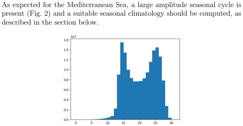
The whole comparison rests on the assumption that errors measured under artificial cloud masks represent what happens under real clouds, even though the paper notes that water under clouds is cooler than clear-sky water, a bias that is smaller at night.
Editorial extensions
If this is right
- The best U-Net64 configuration with four input days is a practical, high-resolution gap-filling method for the Italian seas.
- Adding more than four previous days does not improve reconstruction, so the operational input window can be kept short.
- Splitting the 256x256 domain into four quadrant models improves accuracy, so regional training can outperform a single larger model.
- The method preserves cloud-free pixel values and frontal structures while interpolating under clouds, reducing the smoothing typical of OI products.
- If the reported RMSE advantage holds, data-driven reconstructions could feed operational downstream forcing and reanalysis systems without waiting for multi-day temporal windows.
Reading between the lines
- The same recipe—anomaly target, artificial masks, and a U-Net with a short temporal stack—could transfer to other gridded ocean variables such as chlorophyll or sea ice, where a similar generator protocol is already in use.
- Because error saturates at four input days, the network likely learns a persistence-plus-climatology prior; ablating the temporal channels would show how much of the gain comes from previous days versus spatial context.
- The visible-pixel comparison to L4 is not a true cloud-filling test; the decisive experiment is to compare against independent microwave or in-situ measurements under actual clouds, which the paper does not report.
Signed reviews
Editorial analysis
A structured set of objections, weighed in public.
Referee Report
Summary. This manuscript investigates deep learning models, primarily U-Net and vision transformer architectures, for filling cloud-occluded pixels in nighttime MODIS Aqua sea surface temperature (SST) fields over the Italian seas. The authors describe an artificial cloud generator that superimposes masks from other days to create training and evaluation targets, compare several U-Net/ViT configurations, and report that their best U-Net64 with four days of temporal input outperforms DINCAE and the Copernicus L4 product. The central claim, stated in the abstract, is that the best architecture achieves 50% lower root mean square errors than established gap-filling methods.
Significance. If the headline claim were supported by the evidence, the paper would provide a practical, open-source deep-learning alternative for SST gap filling, with possible operational value for Copernicus Marine products. The manuscript includes useful engineering details: a configurable cloud mask generator, systematic ablation of temporal input length and spatial tiling, and public code availability. However, the reported evaluations do not currently establish the claimed advantage for real cloud-covered pixels: the DINCAE comparison is not a controlled head-to-head, the L4 comparison is restricted to cloud-free pixels, and the synthetic-mask evaluation relies on an assumption of representativeness that the authors themselves flag as a bias risk. The significance of the work therefore hinges on additional validation that is not present.
major comments (5)
- [Abstract and Table 7] The abstract's claim of "50% lower root mean square errors over established gap-filling methods" is contradicted by the paper's own Table 7, which reports U-Net64 RMSE of 0.42 versus DINCAE 0.54, i.e. about 22% lower. Figure 10, the comparison with the L4 product, computes RMSE only on visible (cloud-free) pixels, so it does not measure skill at filling cloud-occluded areas. The central quantitative claim of the paper is therefore not supported by the reported experiments.
- [Section 3.3] The synthetic cloud generator evaluates reconstruction on pixels that are artificially occluded by a mask taken from a different day, and the evaluation region excludes pixels that were already cloudy in the real scene. The paper itself states that "the sea temperature under clouds is usually different from the temperature under a clear sky, but this bias is lower during the night," which is an explicit caveat that the synthetic scenario may not represent real cloud occlusion. No experiment in the manuscript measures RMSE on actual cloud-covered pixels against any ground truth (L4, reanalysis, or in situ data). Consequently, the core claim of improved gap-filling accuracy under real cloud occlusion is not established.
- [Section 2.4] The seasonal climatology used to compute anomalies is described as "the time mean SST across all the 21 years dataset," which includes the 2021-2023 test period. Since the model is trained to predict residuals with respect to this climatology, the test-period mean SST is embedded in the input baseline, leaking information from the test set into both training and evaluation. The climatology should be computed using only data before the test period, and the evaluation should be repeated to assess the impact of this leakage.
- [Section 4.1 and Table 7] The DINCAE comparison is not a controlled head-to-head. Table 7 reports DINCAE RMSE on the Northern Adriatic with fixed artificial masks, MODIS-TERRA data from 2003-2016, and a different evaluation protocol, while the U-Net models are evaluated on the configurable generator over the full Italian seas and a different data period. Differences in region, input data source, mask distribution, and temporal coverage could explain the reported RMSE gap as much as architectural superiority. A valid comparison would require both methods to be evaluated on the same test set and the same occlusion masks.
- [Section 5 and Figure 10] The comparison with the L4 product in Figure 10 is computed over visible sea pixels only, where the U-Net reconstruction coincides with the input L3 values (the model preserves observed values in cloud-free areas). This measures the model's fidelity to its input, not its ability to reconstruct cloud-covered SST. The qualitative comparison in Figure 11 is likewise limited to cloud-free regions. These experiments therefore do not support the conclusion that the U-Net outperforms L4 at gap filling.
minor comments (7)
- [Section 1] The domain coordinates are stated as "latitude between 35.33° and 46.0°E and longitude between 7.92° and 18.58°N"; latitude and longitude units are swapped and should be corrected (latitude in °N, longitude in °E).
- [Section 3.2] "outlied" should be "outlined" in the description of the ViT architecture.
- [Section 3.1] The text contains a typo: "Donwnsamping" should be "Downsampling."
- [Abstract] "Our best-performing architecture show" should be "Our best-performing architecture shows."
- [Table 2] The entries for spatial gradients above 2°C are blank rather than shown as zeros or dashes; the table would be clearer if all cells contained explicit values.
- [Section 5] The sentence "We retrained the model L3S reprocessed data" is missing a preposition; it should read "We retrained the model on L3S reprocessed data."
- [Section 7] "Our selected best model architectures is made of a U-net64 algorithm" should be rephrased, for example "Our selected best model architecture is a U-Net64 algorithm."
Circularity Check
The headline 50% improvement is partially circular: the L4 comparison is computed on visible pixels where the U-Net is designed to copy the input, and the climatology input is fitted on the test period; the core U-Net training itself is a genuine learning benchmark.
-
fitted input called prediction
[Section 2.4 (Seasonal Climatology) and Section 2 (data set description)]
"All nighttime measurements from 7/4/2002 to 12/31/2023 were used. Part of the data, from 7/4/2021 to 12/31/2023, was used for testing purposes. ... Thus, we compute the seasonal climatology as the time mean SST across all the 21 years dataset. Anomalies are then calculated by subtracting from each day the seasonal climatology."
The climatology used as model input is the time mean over the full 21-year dataset, which includes the 2021-2023 test period. Absolute SST is reconstructed as climatology plus predicted anomaly, so the test-period mean SST is already embedded in the input features. The prediction pipeline is therefore fitted, through the climatology, on the very data it is later said to predict; the reported RMSE on reconstructed absolute SST is artificially reduced by this leakage.
-
self definitional
[Section 5, Figure 10 and abstract]
"In Fig. 10, we compare the error by the two different reconstruction methods and the L3 input over visible regions of the sea. ... preserving the integrity of observed values in cloud-free areas."
The model is explicitly designed to preserve observed values in cloud-free areas, and Figure 10 measures error against L3 only on visible regions. On those pixels the U-Net's output is constrained to match the input, so its low RMSE is an identity check, not a test of cloud-gap filling. Comparing this to the L4 OI product, which smooths rather than copies L3, shows only that copying beats smoothing; the claimed superiority over L4 is an artifact of the evaluation region and the model's by-construction input preservation.
full rationale
The core derivation is not fully circular: the U-Net is trained on synthetic cloud occlusions generated following Barth et al. and Goh et al., and its internal comparisons (Tables 5-7) are real inpainting benchmarks computed on artificial masks. No load-bearing self-citation or imported uniqueness theorem is present. However, two steps partially reduce the headline claim to its inputs. First, the seasonal climatology that is subtracted to form the anomaly target is averaged over all 21 years, including the 2021-2023 test interval, so the model's input has seen the test-period mean SST. Second, the L4 comparison in Figure 10 is restricted to visible sea regions, where the model is built to preserve observed values; the low error there is a definitional consequence of the architecture, not a demonstration of skill under clouds. The paper itself flags the transfer risk: the generator is 'a bit unrealistic during testing' and 'risks introducing biases since the sea temperature under clouds is usually different from the temperature under a clear sky.' These are correctly stated limitations, but they mean the abstract's '50% lower root mean square errors over established gap-filling methods' is not established for real cloud-occluded pixels. The DINCAE comparison is external and legitimate as a benchmark, though its different protocol and region make the 22% figure hard to interpret. Overall, partial circularity in the headline evidence warrants a score of 6, not a claim that the entire derivation is empty.
Assumptions & free parameters
free parameters (7)
- Temporal input window length =
4 days
- U-Net64 channel configuration =
[64,128,256,512]
- Spatial tiling into four 128x128 models =
4 quadrants
- Artificial cloud generator thresholds =
>=40% visible sea; >=10% artificial occlusion; >=5% visible sea after masking
- Quality flag cutoff =
flags 0 to 2
- Climatology Gaussian blur scale =
not reported
- Neural network weights =
millions of parameters; U-Net64 has 17,022,273
assumptions (6)
- domain assumption MODIS L3 SST values and quality flags correctly identify cloud-free and cloudy pixels, with negligible contamination from cloud borders.
- ad hoc to paper Artificial occlusion masks sampled from other days are statistically representative of real cloud occlusion, and the nighttime bias between cloud-covered and clear-sky SST is small.
- ad hoc to paper The climatology computed over all years, including the test period, is a valid baseline for test-time reconstruction.
- domain assumption Spatial and temporal persistence plus the seasonal cycle provide sufficient prior information for reconstructing sub-cloud SST.
- domain assumption A model trained on MODIS-Aqua can be applied to Copernicus L3S NRT products with similar cloud-occlusion geometry.
- ad hoc to paper RMSE on visible pixels, where the input L3 SST is known, is a meaningful baseline for comparing gap-filling methods.
Cite this review
Pith. "Pith review of Deep Learning for Sea Surface Temperature Reconstruction under Cloud Occlusion." pith.science (2026). https://pith.science/paper/SYGYRWOW
@misc{pith2026241203413,
  author       = {Pith},
  title        = {Pith review of: Deep Learning for Sea Surface Temperature Reconstruction under Cloud Occlusion},
  year         = {2026},
  howpublished = {\url{https://pith.science/paper/SYGYRWOW}},
  note         = {Machine review of arXiv:2412.03413}
}
read the original abstract
Sea Surface Temperature (SST) reconstructions from satellite images affected by cloud gaps have been extensively documented in the past three decades. Here we describe several Machine Learning models to fill the cloud-occluded areas starting from MODIS Aqua nighttime L3 images. To tackle this challenge, we employed a type of Convolutional Neural Network model (U-net) to reconstruct cloud-covered portions of satellite imagery while preserving the integrity of observed values in cloud-free areas. We demonstrate the outstanding precision of U-net with respect to available products done using OI interpolation algorithms. Our best-performing architecture show 50% lower root mean square errors over established gap-filling methods.
Figures


Figures from the paper (8 more)



Reference graph
Works this paper leans on
-
[1]
write newline
" write newline "" before.all 'output.state := FUNCTION n.dashify 't := "" t empty not t #1 #1 substring "-" = t #1 #2 substring "--" = not "--" * t #2 global.max substring 't := t #1 #1 substring "-" = "-" * t #2 global.max substring 't := while if t #1 #1 substring * t #2 global.max substring 't := if while FUNCTION word.in bbl.in ":" * " " * FUNCTION f...
- [2]
-
[3]
F. P. Bretherton, R. E. Davis, C. Fandry, A technique for objective analysis and design of oceanographic experiments applied to mode-73 23 (7) (1976) 559--582
work page 1976
-
[4]
A. Alvera-Azc \'a rate, A. Barth, D. Sirjacobs, F. Lenartz, J.-M. Beckers, Data interpolating empirical orthogonal functions (dineof): a tool for geophysical data analyses, Mediterranean Marine Science (2011) 5--11
work page 2011
-
[5]
S. Jung, C. Yoo, J. Im, High-resolution seamless daily sea surface temperature based on satellite data fusion and machine learning over kuroshio extension https://doi.org/10.3390/rs14030575, Remote. Sens. 14 (3) (2022) 575. https://doi.org/10.3390/RS14030575 doi:10.3390/RS14030575 . ://doi.org/10.3390/rs14030575
-
[6]
L. Ćatipović, F. Matić, H. Kalinić, Reconstruction methods in oceanographic satellite data observation—a survey https://www.mdpi.com/2077-1312/11/2/340, Journal of Marine Science and Engineering 11 (2) (2023). https://doi.org/10.3390/jmse11020340 doi:10.3390/jmse11020340 . ://www.mdpi.com/2077-1312/11/2/340
-
[7]
B. Buongiorno Nardelli , C. Tronconi, A. Pisano, R. Santoleri, High and ultra-high resolution processing of satellite sea surface temperature data over southern european seas in the framework of myocean project https://www.sciencedirect.com/science/article/pii/S003442571200394X, Remote Sensing of Environment 129 (2013) 1--16. https://doi.org/https://doi.o...
-
[8]
T. M. Chin, J. Vazquez-Cuervo, E. M. Armstrong, A multi-scale high-resolution analysis of global sea surface temperature, Remote sensing of environment 200 (2017) 154--169
work page 2017
Show all 33 references
-
[9]
Fablet, P
R. Fablet, P. H. Viet, R. Lguensat, Data-driven models for the spatio-temporal interpolation of satellite-derived sst fields, IEEE Transactions on Computational Imaging 3 (4) (2017) 647--657
2017
-
[10]
Barth, A
A. Barth, A. Alvera-Azc \'a rate, M. Licer, J.-M. Beckers, Dincae 1.0: a convolutional neural network with error estimates to reconstruct sea surface temperature satellite observations, Geoscientific Model Development 13 (3) (2020) 1609--1622
2020
-
[11]
Barth, A
A. Barth, A. Alvera-Azc \'a rate, C. Troupin, J.-M. Beckers, Dincae 2.0: multivariate convolutional neural network with error estimates to reconstruct sea surface temperature satellite and altimetry observations, Geoscientific Model Development 15 (5) (2022) 2183--2196
2022
-
[12]
Z. Han, Y. He, G. Liu, W. Perrie, Application of dincae to reconstruct the gaps in chlorophyll-a satellite observations in the south china sea and west philippine sea, Remote Sensing 12 (3) (2020) 480
2020
-
[13]
E. Goh, A. R. Yepremyan, J. Wang, B. Wilson, Maesstro: Masked autoencoders for sea surface temperature reconstruction under occlusion, EGUsphere 2023 (2023) 1--20
2023
-
[14]
Iizuka, E
S. Iizuka, E. Simo - Serra, H. Ishikawa, Globally and locally consistent image completion https://doi.org/10.1145/3072959.3073659, ACM Trans. Graph. 36 (4) (2017) 107:1--107:14. https://doi.org/10.1145/3072959.3073659 doi:10.1145/3072959.3073659 . ://doi.org/10.1145/3072959.3073659
2017
-
[15]
G. Liu, F. A. Reda, K. J. Shih, T. Wang, A. Tao, B. Catanzaro, Image inpainting for irregular holes using partial convolutions https://doi.org/10.1007/978-3-030-01252-6\_6, in: Computer Vision - ECCV 2018 - 15th European Conference, Munich, Germany, September 8-14, 2018, Proce...
2018 doi
-
[16]
H. Liu, B. Jiang, Y. Song, W. Huang, C. Yang, Rethinking image inpainting via a mutual encoder-decoder with feature equalizations https://doi.org/10.1007/978-3-030-58536-5\_43, in: Computer Vision - ECCV 2020 - 16th European Conference, Glasgow, UK, August 23-28, 2020, Proceed...
2020 doi
-
[17]
J. Peng, D. Liu, S. Xu, H. Li, https://openaccess.thecvf.com/content/CVPR2021/html/Peng\_Generating\_Diverse\_Structure\_for\_Image\_Inpainting\_With\_Hierarchical\_VQ-VAE\_CVPR\_2021\_paper.html Generating diverse structure for image inpainting with hierarchical VQ-VAE , in: ...
2021
-
[18]
Z. Wan, J. Zhang, D. Chen, J. Liao, High-fidelity pluralistic image completion with transformers https://doi.org/10.1109/ICCV48922.2021.00465, in: 2021 IEEE/CVF International Conference on Computer Vision, ICCV 2021, Montreal, QC, Canada, October 10-17, 2021, 2021, pp. 4672--4...
2021
-
[19]
Zheng, T
C. Zheng, T. Cham, J. Cai, D. Q. Phung, Bridging global context interactions for high-fidelity image completion https://doi.org/10.1109/CVPR52688.2022.01122, in: IEEE/CVF Conference on Computer Vision and Pattern Recognition, CVPR 2022, New Orleans, LA, USA, June 18-24, 2022, ...
2022
-
[20]
J. Jain, Y. Zhou, N. Yu, H. Shi, Keys to better image inpainting: Structure and texture go hand in hand https://doi.org/10.1109/WACV56688.2023.00029, in: IEEE/CVF Winter Conference on Applications of Computer Vision, WACV 2023, Waikoloa, HI, USA, January 2-7, 2023, 2023, pp. 2...
2023
-
[21]
P. J. Werdell, B. A. Franz, S. W. Bailey, G. C. Feldman, E. Boss, V. E. Brando, M. Dowell, T. Hirata, S. J. Lavender, Z. Lee, et al., Generalized ocean color inversion model for retrieving marine inherent optical properties, Applied optics 52 (10) (2013) 2019--2037
2013
-
[22]
Pinardi, M
N. Pinardi, M. Zavatarelli, M. Adani, G. Coppini, C. Fratianni, P. Oddo, S. Simoncelli, M. Tonani, V. Lyubartsev, S. Dobricic, et al., Mediterranean sea large-scale low-frequency ocean variability and water mass formation rates from 1987 to 2007: A retrospective analysis, Prog...
2015
-
[23]
Ronneberger, P
O. Ronneberger, P. Fischer, T. Brox, U-net: Convolutional networks for biomedical image segmentation, in: Medical Image Computing and Computer-Assisted Intervention - MICCAI 2015 - 18th International Conference Munich, Germany, October 5 - 9, 2015, Proceedings, Part III , 2015...
2015
-
[24]
Dosovitskiy, L
A. Dosovitskiy, L. Beyer, A. Kolesnikov, D. Weissenborn, X. Zhai, T. Unterthiner, M. Dehghani, M. Minderer, G. Heigold, S. Gelly, J. Uszkoreit, N. Houlsby, An image is worth 16x16 words: Transformers for image recognition at scale https://openreview.net/forum?id=YicbFdNTTy, in...
2021
-
[25]
J. Ho, A. Jain, P. Abbeel, Denoising diffusion probabilistic models https://proceedings.neurips.cc/paper/2020/hash/4c5bcfec8584af0d967f1ab10179ca4b-Abstract.html, in: H. Larochelle, M. Ranzato, R. Hadsell, M. Balcan, H. Lin (Eds.), Advances in Neural Information Processing Sys...
2020
-
[26]
J. Song, C. Meng, S. Ermon, Denoising diffusion implicit models https://openreview.net/forum?id=St1giarCHLP, in: 9th International Conference on Learning Representations, ICLR 2021, Virtual Event, Austria, May 3-7, 2021, OpenReview.net, 2021. ://openreview.net/forum?id=St1giarCHLP
2021
-
[27]
Vaswani, N
A. Vaswani, N. Shazeer, N. Parmar, J. Uszkoreit, L. Jones, A. N. Gomez, L. Kaiser, I. Polosukhin, Attention is all you need https://proceedings.neurips.cc/paper/2017/hash/3f5ee243547dee91fbd053c1c4a845aa-Abstract.html, in: Advances in Neural Information Processing Systems 30: ...
2017
-
[28]
Vaswani, N
A. Vaswani, N. Shazeer, N. Parmar, J. Uszkoreit, L. Jones, A. N. Gomez, L. u. Kaiser, I. Polosukhin, Attention is all you need https://proceedings.neurips.cc/paper_files/paper/2017/file/3f5ee243547dee91fbd053c1c4a845aa-Paper.pdf, in: I. Guyon, U. V. Luxburg, S. Bengio, H. Wall...
2017
-
[29]
Merizzi, A
F. Merizzi, A. Asperti, S. Colamonaco, https://doi.org/10.1007/s00521-024-10139-9 Wind speed super-resolution and validation: from ERA5 to CERRA via diffusion models , Neural Computing and Applications (2024). ://doi.org/10.1007/s00521-024-10139-9
2024 doi
-
[30]
Asperti, F
A. Asperti, F. Merizzi, A. Paparella, G. Pedrazzi, M. Angelinelli, S. Colamonaco, Precipitation nowcasting with generative diffusion models, Applied Intelligence To appear (2024)
2024
-
[31]
Szegedy, W
C. Szegedy, W. Liu, Y. Jia, P. Sermanet, S. E. Reed, D. Anguelov, D. Erhan, V. Vanhoucke, A. Rabinovich, Going deeper with convolutions https://doi.org/10.1109/CVPR.2015.7298594, in: IEEE Conference on Computer Vision and Pattern Recognition, CVPR 2015, Boston, MA, USA, June 7...
2015
-
[32]
J. Park, S. Woo, J. Lee, I. S. Kweon, http://bmvc2018.org/contents/papers/0092.pdf BAM: bottleneck attention module , in: British Machine Vision Conference 2018, BMVC 2018, Newcastle, UK, September 3-6, 2018, 2018, p. 147. ://bmvc2018.org/contents/papers/0092.pdf
2018
-
[33]
S. Woo, J. Park, J. Lee, I. S. Kweon, https://doi.org/10.1007/978-3-030-01234-2\_1 CBAM: convolutional block attention module , in: Computer Vision - ECCV 2018 - 15th European Conference, Munich, Germany, September 8-14, 2018, Proceedings, Part VII , 2018, pp. 3--19. https://d...
2018 doi
Reviewed August 11, 2026 · model on record in the stance chip above.
Discussion (0). Continue with ORCID to comment.