REVIEW 4 major objections 6 minor 16 references
Estimating Large Global Significances with a New Monte Carlo Extrapolation Method
T0 review · 4 major / 6 minor · reviewed 2026-08-10 · deepseek-v4-flash
Pith's one-line read A chi-squared fit to the tail of toy-MC likelihood ratios estimates large global significances that direct counting cannot reach.
desk verdict Practical tail-extrapolation trick for global significances, validated at 4σ but with no propagated uncertainty; worth reviewing, needs a robustness analysis. read the letter →
The pith
A machine-rendered reading of the paper's core claim, the machinery that carries it, and where it could break.
The reading
What carries the argument
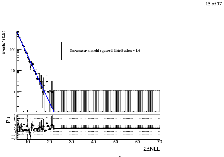
The load-bearing object is the $χ^{2}$ distribution used as a tail model for the log-likelihood ratio 2×(L0−L1) from background-only toys. A single parameter n, the number of degrees of freedom, is fitted to the simulated tail above a ratio of 15; for the three test cases the fitted values are n≈2.5, 2.6, and 1.6. Because the $χ^{2}$ tail is linear on a log scale at large values, a fit to ratios between 15 and 70 can be integrated to predict the number of toys that would exceed much larger ratios such as 28 or 58, which are the values corresponding to 5.3σ and 7.6σ local significances. The p-value is the predicted count above the observed ratio divided by the total number of toys (counted below 15 plus integrated above 15), and the final significance is read off a symmetric Gaussian.
What would settle it
Generate a very large background-only toy sample for the CDF Y(4140) setup, directly count the number of toys with likelihood ratio above 28, and compare that count with the prediction from the chi-squared tail fitted above 15; a statistically significant mismatch between the direct count and the extrapolated count would show that the tail model fails at high ratios.
Extended reading notes
Core claim
The central claim is that, for background-only toy Monte Carlo experiments, the distribution of the log-likelihood ratio 2×(L0−L1) has a tail that is well described by a $χ^{2}$ distribution with a single fitted degrees-of-freedom parameter, and that this tail can therefore be extrapolated far beyond the largest values actually simulated. The method works as follows: simulate a modest number of toys, split the likelihood-ratio distribution at a threshold (15 in this paper, chosen after trial and error), count toys below the threshold, fit a $χ^{2}$ function to the tail above it, and integrate the fitted function to obtain the expected number of toys above the likelihood ratio observed in real data. That expected count divided by the total number of toys is the p-value, converted to a Gaussian significance. On CDF's Y(4140), the extrapolated p-value 2.89×$10^{{-5}}$ gives 4.0σ versus 2.50×$10^{{-5}}$ and 4.1σ from direct counting; on CMS's Y(4140), whose local significance is 7.6σ, the method yields a global significance of 6.6σ (with the alternative upcrossing method giving 6.8σ), and the same procedure on ATLAS's χb(3P) yields 5.7σ (with the alternative giving 5.6σ).
Load-bearing premise
The argument depends on the fitted chi-squared tail continuing to describe the true fluctuation distribution far above the range where it was fitted, so the extrapolation to ratios like 28 or 58 is trustworthy; if the true tail falls off differently, the estimated global significance is biased.
Editorial extensions
If this is right
- Global significances for local significances above 5σ can be evaluated with a few hundred thousand toy experiments instead of the 10^14 or more that direct counting would require.
- The extrapolated global significance agrees with direct counting to within 0.1σ on the CDF Y(4140) case, and with the alternate upcrossing method to within 0.2σ on the CMS and ATLAS cases.
- The method is transferable across different experiments and mass spectra, as demonstrated on CDF, CMS, and ATLAS data with different signal and background models.
- For signals below 5σ, the same simulation machinery lets analyzers estimate the probability of reaching 5σ with additional data, as illustrated for the CMS X(7100) candidate.
- Because it uses only the tail of the fitted distribution, the method also works when the observed significance is so high that no single toy experiment reaches it.
Reading between the lines
- The choice of the tail threshold (15) is heuristic and tuned by trial and error; a principled, data-driven way to pick it would make the method more robust, a step the paper does not take.
- In the CMS case the two cross-checked methods agree to 0.2σ, yet their p-values differ by an order of magnitude; near decision thresholds like 3σ or 5σ such differences would matter, so the method is safest for the high-significance regime it targets.
- One could stress-test the chi-squared tail assumption by applying the extrapolation to a search whose exact global significance is computable analytically, such as a single-channel Gaussian field, and checking whether the fitted tail remains valid as the extrapolation distance grows.
- The same tail-fitting logic might extend beyond mass-spectrum searches to any likelihood-ratio scan, provided the asymptotic chi-squared behavior of the test statistic holds.
Editorial analysis
A structured set of objections, weighed in public.
Referee Report
Summary. The paper describes a new 'extrapolation' method for estimating global significances in particle physics searches. The method generates a modest number of background-only toy Monte Carlo experiments, fits a chi-square distribution to the upper tail (starting at 2ΔLLR = 15) of the likelihood-ratio distribution, and integrates the fitted function to estimate the expected number of toys above a high threshold. The authors validate the method on CDF's Y(4140) by comparing with direct counting (4.0σ vs 4.1σ), cross-check it with the Gross-Vitells (G-V) method, and apply it to CMS's Y(4140) (6.6σ) and ATLAS's χb(3P) (5.7σ), where direct counting is impractical.
Significance. If the method's accuracy at large extrapolation distances were established, it would be a practically valuable, easy-to-implement alternative to brute-force toy MC for global significances beyond 5σ, avoiding samples of order 10^14. The paper includes a useful demonstration of the conventional counting method on the CMS X(7100) case and a reproducible simulation setup. The CDF validation is encouraging: the extrapolated tail expectation above 2ΔLLR = 28 (10.4 toys) agrees with the direct count (9 toys) within 0.1σ. However, the current evidence for predictive power in the advertised high-significance regime is limited: the validation is in-sample (the tail threshold is chosen on the same dataset), and the only high-significance cross-check (G-V) differs by a factor of about 2.6 in p-value for CMS. The method's usefulness depends on quantifying the uncertainty of tail extrapolation.
major comments (4)
- [Sec. 4.3, Table 2] No uncertainties are quoted for the extrapolated global significances in Table 2 (CMS 6.6σ, ATLAS 5.7σ). In the CMS case the extrapolated p-value is 1.58×10^-11 from an expected count of 4.30×10^-6 toys above 2ΔLLR = 58, and a small change in the fitted degrees-of-freedom parameter n = 2.6 (quoted without uncertainty) or in the tail threshold would change this expectation by orders of magnitude. The authors should propagate the fit uncertainty in n and the finite-toy uncertainty to the extrapolated p-value, and quote an uncertainty on the final significance. Without this, the claim that the method 'gives good estimation' is not quantitatively assessable.
- [Sec. 4.2.4] The tail-fit threshold of 15 is chosen 'after some trial and error' on the CDF toy sample, and the same 359,758-toy sample is then used to validate the method at 2ΔLLR = 28. This is an in-sample validation, not an out-of-sample prediction. The central claim of predictive power for CMS (threshold 58) and ATLAS (threshold 36) requires either an out-of-sample test, a closure test at an intermediate threshold where direct counting is feasible, or a systematic scan of the threshold and fit range demonstrating that the extrapolated significance is stable. The current presentation does not provide such evidence.
- [Sec. 4.2.4 and Sec. 4.3] The paper provides no theoretical or empirical justification that a chi-square distribution with a single fitted degree-of-freedom parameter describes the extreme tail of the scanned 2ΔLLR distribution over many orders of magnitude. In the CMS case the extrapolated expected count is about 10^9 below the tail-integral anchor at 15, so the tail-shape assumption is load-bearing. The authors should test this assumption concretely, for example by using a larger toy sample at an intermediate threshold, comparing with an alternative parametric tail (e.g., exponential or generalized Pareto), or varying the fit threshold over a plausible range and showing that the extrapolated significance is robust.
- [Sec. 4.3] In the only high-significance regime where an independent cross-check exists, the extrapolation method and the G-V method disagree by a factor of 2.6 in p-value (1.58×10^-11 vs 6.16×10^-12). The text dismisses this as a 0.2σ difference, but for a claim of 'good estimation' the relevant quantity is the p-value, and a factor 2.6 is large. Moreover, the G-V input <N(c0)> = 18.80 ± 2.75 implies a substantial uncertainty in the G-V p-value, which is not propagated either. The authors should quantify the accuracy target of the method and either reconcile the discrepancy or include it as an uncertainty.
minor comments (6)
- [Sec. 4.2.4] The fit range is described both as [15,70] and as 'above 15' when computing the total toy count; please clarify whether the normalization integral of the fitted chi-square distribution is taken over [15,70] or [15,∞).
- [Sec. 4.2.4] The quoted values of the fitted degrees-of-freedom parameter (n = 2.5, 2.6, 1.6) are given without fit uncertainties; please report them.
- [Sec. 4.4] The statement 'After extrapolation, we obtained a result of (3.53 ± 0.07) × 10^-04' does not define what the quantity is or where the uncertainty comes from; please state that this is the expected number of toys above 2ΔLLR = 36 and explain the uncertainty's source.
- [Footnote 1, Sec. 4.3] The footnote 'We became aware of a relevant paper [15] after publication, thus a comparison with it cannot be done' is a self-acknowledged missing comparison; the authors should either add the comparison or justify its omission in the main text.
- [Abstract and Sec. 2.3] The phrase 'assuming symmetrical Gaussian distributions' is imprecise; the conversion uses the one-sided upper tail of a standard normal distribution, not a two-sided symmetric interval.
- [Sec. 4.3] The sentence 'their corresponding p-values differ by an order of magnitude, making error calculation challenging' should be elaborated or removed; an order-of-magnitude difference is precisely what needs to be explained when claiming good estimation.
Circularity Check
No significant circularity: the extrapolated tail count is not an input to the chi-squared fit, and the CDF direct-count and G-V comparisons provide independent checks.
full rationale
The paper's central quantity—the expected number of toy experiments above a target likelihood ratio—is obtained by integrating a chi-squared distribution fitted to the observed tail above ratio 15 (Sec 4.2.4). The target thresholds (28, 58, 36) are not used as fit constraints, and the number of toys above the target is not an input to the fit; it is the output of the integral. In the CDF validation, the extrapolated expectation 10.4 is compared with the independently counted 9 events above 28, which is a separate estimator on the same toy sample and therefore a genuine cross-check, not a quantity forced by construction. The post-hoc choice of the fit threshold ('after some trial and error') and the in-sample location of the threshold 28 within the fit interval [15,70] are statistical robustness concerns, not circularity. The CMS and ATLAS results are benchmarked against the independent Gross-Vitells method, and agreement within 0.1-0.2 sigma is reported. The only self-citation is Ref [11] (Yi, Spiegel, Hu) used in Sec. 3 to describe the conventional counting method; this is not load-bearing for the new extrapolation claim or for its validation. No step in the derivation reduces by definition to its own inputs, no fitted parameter is renamed as a prediction, and no uniqueness theorem is imported from the authors' prior work. The appropriate finding is a low circularity score reflecting the minor non-load-bearing self-citation.
Assumptions & free parameters
free parameters (2)
- chi-squared degrees of freedom n =
2.5 (CDF), 2.6 (CMS), 1.6 (ATLAS)
- tail fit threshold =
15 (likelihood ratio)
assumptions (3)
- domain assumption The high tail of the toy MC log-likelihood ratio distribution is well described by a chi-squared distribution with unknown degrees of freedom.
- domain assumption The background-only toy MC samples correctly model the null hypothesis, including known resonances and phase-space backgrounds.
- standard math Converting p-values to Gaussian sigmas via a one-sided symmetric Gaussian integral is appropriate.
Cite this review
Pith. "Pith review of Estimating Large Global Significances with a New Monte Carlo Extrapolation Method." pith.science (2026). https://pith.science/paper/HQPAFZ4S
@misc{pith2026241220777,
  author       = {Pith},
  title        = {Pith review of: Estimating Large Global Significances with a New Monte Carlo Extrapolation Method},
  year         = {2026},
  howpublished = {\url{https://pith.science/paper/HQPAFZ4S}},
  note         = {Machine review of arXiv:2412.20777}
}
read the original abstract
In particle physics, it is needed to evaluate the possibility that excesses of events in mass spectra are due to statistical fluctuations as quantified by the standards of local and global significances. Without prior knowledge of a particle's mass, it is especially critical to estimate its global significance. The usual approach is to count the number of times a significance limit is exceeded in a collection of simulated Monte Carlo (MC) 'toy experiments.' To demonstrate this conventional method for global significance, we performed simulation studies according to a recent Compact Muon Solenoid (CMS) result to show its effectiveness. However, this counting method is not practical for computing large global significances. To address this problem, we developed a new 'extrapolation' method to evaluate the global significance. We compared the global significance estimated by our new method with that of the conventional approach, and verified its feasibility and effectiveness. This method is also applicable for cases where only small toy MC samples are available. In this approach, the significance is calculated based on p-values, assuming symmetrical Gaussian distributions.
Figures


Figures from the paper (12 more)



Reference graph
Works this paper leans on
-
[1]
New Structures in the J/ψJ/ψ Mass Spectrum in Proton-Proton Collisions at √s = 13 TeV .Phys
CMS Collaboration. New Structures in the J/ψJ/ψ Mass Spectrum in Proton-Proton Collisions at √s = 13 TeV .Phys. Rev. Lett. 2024, 132, 111901
work page 2024
-
[2]
Experimental Road to a Charming Family of Tetraquarks
Zhu, F.; Bauer, G.; Yi, K. Experimental Road to a Charming Family of Tetraquarks... and Beyond.Chin. Phys. Lett. 2024, 41, 111201
work page 2024
-
[3]
Liu, X. Four-Charm-Quark Matter from the CMS Collaboration as a witness of the development of high- precision hadron spectroscopy. Sci. Bull. 2024, 69, 2802-2803
work page 2024
-
[4]
Evidence for a Narrow Near-Threshold Structure in the J/ψϕ Mass Spectrum in B+ → J/ψϕK+ Decays
CDF Collaboration. Evidence for a Narrow Near-Threshold Structure in the J/ψϕ Mass Spectrum in B+ → J/ψϕK+ Decays. Phys. Rev. Lett. 2009, 102, 242002
work page 2009
-
[5]
Experimental review of structures in the J/ψϕ mass spectrum
Yi, K. Experimental review of structures in the J/ψϕ mass spectrum. Int. J. Mod. Phys. A 2013, 28, 1330020
work page 2013
-
[6]
Observation of the Y(4140) Structure in the J/ψϕ Mass Spectrum in B± → J/ψϕK± Decays
CDF Collaboration. Observation of the Y(4140) Structure in the J/ψϕ Mass Spectrum in B± → J/ψϕK± Decays. Mod. Phys. Lett. A 2017, 32, 1750139
work page 2017
-
[7]
Observation of a peaking structure in the J/ψϕ mass spectrum from B± → J/ψϕK± decays
CMS Collaboration. Observation of a peaking structure in the J/ψϕ mass spectrum from B± → J/ψϕK± decays. Phys. Lett. B 2014, 734, 261-281
work page 2014
-
[8]
Trial factors for the look elsewhere effect in high energy physics
Gross, E.; Vitells, O. Trial factors for the look elsewhere effect in high energy physics. Eur. Phys. J. C 2010, 70, 525-530
work page 2010
Show all 16 references
-
[9]
Observation of a new χb state in radiative transitions to Υ(1S) and Υ(2S) at ATLAS
ATLAS Collaboration. Observation of a new χb state in radiative transitions to Υ(1S) and Υ(2S) at ATLAS. Phys. Rev. Lett. 2012, 108, 152001
2012
-
[10]
Probability and Statistics in Experimental Physics ; Springer Science & Business Media: Berlin/Heidelberg, Germany, 1992
Byron, P .R. Probability and Statistics in Experimental Physics ; Springer Science & Business Media: Berlin/Heidelberg, Germany, 1992
1992
-
[11]
A global significance evaluation method using simulated events
Yi, K.J.; Spiegel, L.; Hu, Z. A global significance evaluation method using simulated events. arXiv 2023, arXiv:2310.14317
2023 arXiv
-
[12]
Observation of new structures in the J/ψJ/ψ mass spectrum in pp collisions at √s = 13 TeV
CMS Collaboration. Observation of new structures in the J/ψJ/ψ mass spectrum in pp collisions at √s = 13 TeV . CMS-PAS-BPH-21-003. 2022. Available online: https://cds.cern.ch/record/2815336 (accessed on 9 July 2022). 17 of 17
2022
-
[13]
ROOT: An object oriented data analysis framework
Brun, R.; Rademakers, F. ROOT: An object oriented data analysis framework. Nucl. Inst. Meth. Phys. Res. 1997, 389, 81-86
1997
-
[14]
Observation of New Structure in the J/ψJ/ψ Mass Spectrum in Proton-Proton Collisions at √s = 13 TeV
CMS Collaboration. Observation of New Structure in the J/ψJ/ψ Mass Spectrum in Proton-Proton Collisions at √s = 13 TeV . 2023. Available online: https://doi.org/10.17182/hepdata.141028 (accessed on 13 July 2023)
2023 doi
-
[15]
The profile likelihood ratio and the look elsewhere effect in high energy physics
Ranucci, G. The profile likelihood ratio and the look elsewhere effect in high energy physics. Nucl. Inst. Meth. Phys. Res. A 2012, 661, 77-85
2012
-
[16]
Review of Particle Physics
Particle Data Group. Review of Particle Physics. Phys. Lett. B 2008, 667, 1
2008
Reviewed August 10, 2026 · model on record in the stance chip above.
Discussion (0). Continue with ORCID to comment.