Simulating quantum circuits with arbitrary local noise using Pauli Propagation
Pith reviewed 2026-05-23 04:38 UTC · model grok-4.3
The pith
Typical quantum circuits under any local noise admit polynomial-time classical simulation of expectation values via Pauli propagation with truncation.
A machine-rendered reading of the paper's core claim, the machinery that carries it, and where it could break.
Core claim
With high probability over the circuit gates choice, Pauli propagation algorithms with tailored truncation strategies achieve an inversely polynomially small simulation error for estimating expectation values of arbitrary observables on typical quantum circuits under any incoherent local noise. This holds for arbitrary circuit topologies under the assumption that the distribution of each circuit layer is invariant under single-qubit random gates. Under the same minimal assumptions, most noisy circuits can be truncated to an effective logarithmic depth for the task of estimating expectation values of observables.
What carries the argument
Pauli propagation algorithms with tailored truncation strategies that discard low-weight or heavily damped Pauli paths while propagating operators through the noisy circuit.
If this is right
- Expectation values of arbitrary observables on typical noisy circuits become classically estimable in polynomial time.
- The same invariance condition implies that most circuits admit an effective logarithmic-depth truncation for this estimation task.
- The guarantees extend to non-unital noise and dephasing on arbitrary topologies.
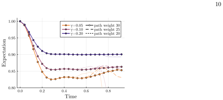
- Numerical checks on 6x6 and 11x11 lattices confirm practical performance under amplitude damping and dephasing.
Where Pith is reading between the lines
- Quantum advantage arguments for noisy circuits may have to target worst-case or specially constructed ensembles rather than typical ones.
- The truncation approach could be tested on other observables or combined with tensor-network methods for further scaling.
- If the invariance condition can be relaxed while preserving the high-probability bound, the result would apply to an even wider class of hardware-relevant circuits.
Load-bearing premise
The distribution of each circuit layer is invariant under single-qubit random gates.
What would settle it
An explicit ensemble of circuits obeying the layer-invariance condition for which the Pauli-propagation truncation error remains larger than any inverse polynomial for some observable and some system size.
Figures


read the original abstract
We present a polynomial-time classical algorithm for estimating expectation values of arbitrary observables on typical quantum circuits under any incoherent local noise, including non-unital or dephasing. Although previous research demonstrated that some carefully designed quantum circuits affected by non-unital noise cannot be efficiently simulated, we show that this does not apply to average-case circuits, as these can be efficiently simulated using Pauli-path methods. Specifically, we prove that, with high probability over the circuit gates choice, Pauli propagation algorithms with tailored truncation strategies achieve an inversely polynomially small simulation error. This result holds for arbitrary circuit topologies and for any local noise, under the assumption that the distribution of each circuit layer is invariant under single-qubit random gates. Under the same minimal assumptions, we also prove that most noisy circuits can be truncated to an effective logarithmic depth for the task of {estimating} expectation values of observables, thus generalizing prior results to a significantly broader class of circuit ensembles. We further numerically validate our algorithm with simulations on a $6\times6$ lattice of qubits under the effects of amplitude damping and dephasing noise, as well as real-time dynamics on an $11\times11$ lattice of qubits affected by amplitude damping.
Editorial analysis
A structured set of objections, weighed in public.
Referee Report
Summary. The manuscript presents a polynomial-time classical algorithm using Pauli propagation with tailored truncation strategies to estimate expectation values of arbitrary observables on typical quantum circuits subject to arbitrary incoherent local noise. It proves that, with high probability over random gate choices, the simulation error is inversely polynomially small, under the assumption that each circuit layer distribution is invariant under single-qubit random gates. The result applies to arbitrary topologies and generalizes prior logarithmic-depth truncation results; numerical validation is provided on 6×6 lattices with amplitude damping and dephasing, and 11×11 lattices with amplitude damping.
Significance. If the central claims hold, the work is significant for establishing efficient classical simulability of average-case noisy quantum circuits under any local incoherent noise, in contrast to known worst-case hardness results. The high-probability guarantees over circuit ensembles, the minimal invariance assumption, and the numerical validation on moderately sized lattices are strengths that support broader applicability of Pauli-path methods.
major comments (3)
- [Abstract and main theorem] Abstract and the statement of the main theorem: the high-probability inverse-polynomial error bound is derived using the layer-invariance assumption to obtain concentration on the weight distribution of propagated Pauli operators after noise application. The proof sketch should explicitly derive the tail bound on surviving paths (e.g., via the averaged noise channel) to confirm that the truncation error remains 1/poly when the invariance holds; without this step the generalization to arbitrary local noise is not fully load-bearing.
- [Truncation strategy section] Section on truncation strategy (likely §3 or §4): the claim that most noisy circuits can be truncated to effective logarithmic depth for expectation-value estimation routes through the same invariance to control path magnitudes. A concrete calculation showing how the invariance implies the required tail decay would strengthen the result; currently the connection between the assumption and the log-depth claim is stated but not derived in detail.
- [Numerical validation] Numerical validation section (6×6 lattice results): the reported simulation errors under amplitude damping should be plotted or tabulated against circuit depth or system size to allow direct comparison with the theoretical 1/poly scaling; without this quantitative link the numerics do not yet confirm the high-probability bound.
minor comments (2)
- [Abstract] The abstract states the result holds for 'arbitrary circuit topologies'; the main text should clarify whether the invariance assumption is required uniformly across all layers or can be relaxed for some layers.
- [Preliminaries] Notation for the noise channel and Pauli operators should be introduced consistently before the main theorem to improve readability.
Simulated Author's Rebuttal
We thank the referee for their careful reading, positive assessment of the significance, and constructive suggestions. We address each major comment below and will incorporate the clarifications in the revised manuscript.
read point-by-point responses
-
Referee: [Abstract and main theorem] Abstract and the statement of the main theorem: the high-probability inverse-polynomial error bound is derived using the layer-invariance assumption to obtain concentration on the weight distribution of propagated Pauli operators after noise application. The proof sketch should explicitly derive the tail bound on surviving paths (e.g., via the averaged noise channel) to confirm that the truncation error remains 1/poly when the invariance holds; without this step the generalization to arbitrary local noise is not fully load-bearing.
Authors: We agree that expanding the proof sketch will strengthen the presentation. In the revised manuscript we will add an explicit derivation of the tail bound on surviving paths, obtained by applying the averaged noise channel under the layer-invariance assumption; this step will directly confirm that the truncation error remains inverse-polynomial with high probability over the circuit ensemble. revision: yes
-
Referee: [Truncation strategy section] Section on truncation strategy (likely §3 or §4): the claim that most noisy circuits can be truncated to effective logarithmic depth for expectation-value estimation routes through the same invariance to control path magnitudes. A concrete calculation showing how the invariance implies the required tail decay would strengthen the result; currently the connection between the assumption and the log-depth claim is stated but not derived in detail.
Authors: We concur that a self-contained calculation will clarify the argument. We will insert a concrete derivation in the truncation-strategy section that shows how single-qubit random-gate invariance produces the required exponential tail decay on Pauli-path magnitudes, thereby rigorously justifying the effective logarithmic-depth truncation for typical circuits. revision: yes
-
Referee: [Numerical validation] Numerical validation section (6×6 lattice results): the reported simulation errors under amplitude damping should be plotted or tabulated against circuit depth or system size to allow direct comparison with the theoretical 1/poly scaling; without this quantitative link the numerics do not yet confirm the high-probability bound.
Authors: We accept that the current numerical section would benefit from explicit scaling plots. In the revision we will add figures and tables that display the observed simulation errors versus circuit depth and lattice size for both amplitude-damping and dephasing noise, allowing direct visual comparison with the predicted 1/poly scaling. revision: yes
Circularity Check
No circularity; result conditioned on explicit external invariance assumption
full rationale
The paper's central high-probability bound and logarithmic-depth truncation are derived under the stated assumption that each circuit layer distribution is invariant under single-qubit random gates. This assumption is presented as minimal and external rather than derived internally. No equations reduce a prediction to a fitted parameter by construction, no self-citation chain is load-bearing for the uniqueness or derivation, and no ansatz is smuggled via prior work. The derivation is therefore self-contained against the given assumptions and random-gate ensemble, consistent with a non-circular analysis.
Axiom & Free-Parameter Ledger
axioms (1)
- domain assumption The distribution of each circuit layer is invariant under single-qubit random gates.
Lean theorems connected to this paper
-
IndisputableMonolith/Foundation/AbsoluteFloorClosure.leanreality_from_one_distinction unclear?
unclearRelation between the paper passage and the cited Recognition theorem.
we prove that, with high probability over the circuit gates choice, Pauli propagation algorithms with tailored truncation strategies achieve an inversely polynomially small simulation error... under the assumption that the distribution of each circuit layer is invariant under single-qubit random gates
-
IndisputableMonolith/Cost/FunctionalEquation.leanwashburn_uniqueness_aczel unclear?
unclearRelation between the paper passage and the cited Recognition theorem.
EV ∼D ‖N†⊗n(V† P V)‖²_F ≤ (χ²_D(N))^{|P|}
-
IndisputableMonolith/Foundation/AlexanderDuality.leanalexander_duality_circle_linking unclear?
unclearRelation between the paper passage and the cited Recognition theorem.
any local noise effectively truncates typical circuits to a logarithmic depth
What do these tags mean?
- matches
- The paper's claim is directly supported by a theorem in the formal canon.
- supports
- The theorem supports part of the paper's argument, but the paper may add assumptions or extra steps.
- extends
- The paper goes beyond the formal theorem; the theorem is a base layer rather than the whole result.
- uses
- The paper appears to rely on the theorem as machinery.
- contradicts
- The paper's claim conflicts with a theorem or certificate in the canon.
- unclear
- Pith found a possible connection, but the passage is too broad, indirect, or ambiguous to say the theorem truly supports the claim.
Forward citations
Cited by 9 Pith papers
-
SAFE ma-QAOA: Surrogate-Assisted and Fine-Tuning Enhanced Multi-Angle QAOA with Parameter Distillation
SAFE ma-QAOA achieves 64.3% fewer active parameters and 94.5% lower estimated QPU workload via surrogate pre-training and parameter distillation on Sherrington-Kirkpatrick, 2D spin glass, and Max-Cut instances.
-
Noise-induced Simulability Transition from Operator Scrambling
Above a critical noise strength, operator scrambling in random circuits is suppressed leading to classical simulability; below it, simulation stays exponentially hard.
-
Efficient simulation of noisy IQP circuits with amplitude-damping noise
A classical polynomial-time sampler exists for the output distribution of amplitude-damped IQP circuits with logarithmic depth and arbitrary l-local diagonal gates.
-
Bra-ket entanglement, an indicator bridging entanglement, magic, and coherence
Bra-ket entanglement indicates a shift from coherence-dominated to magic-dominated entanglement generation as its value increases.
-
Fast, accurate, high-resolution simulation of large-scale Fermi-Hubbard models on a digital quantum processor
A digital quantum processor simulates the 1D Fermi-Hubbard model on up to 120 qubits, observing spin-charge separation and achieving quantitative agreement with TDVP while running up to 3000 times faster in wall-clock...
-
QCommute: a tool for symbolic computation of nested commutators in quantum many-body spin-1/2 systems
QCommute is a new C++ tool for algebraic symbolic computation of nested commutators in quantum spin-1/2 many-body systems on hypercubic lattices in the thermodynamic limit.
-
Sampling (noisy) quantum circuits through randomized rounding
Gaussian randomized rounding on two-qubit marginals of depth-D circuits with local depolarizing noise p yields samples whose expected Max-Cut cost matches the noisy quantum device up to an approximation ratio of 1-O[(1-p)^D].
-
Mind the gaps: The fraught road to quantum advantage
The authors identify four transitions needed to reach fault-tolerant application-scale quantum computing from current NISQ devices.
-
Mind the gaps: The fraught road to quantum advantage
The paper identifies four key hurdles in the transition from NISQ to FASQ quantum computers and argues that targeting them will accelerate progress toward useful quantum advantage.
Reference graph
Works this paper leans on
- [1]
-
[2]
Z. Zhou, R. Sitler, Y. Oda, K. Schultz, and G. Quiroz, Quantum crosstalk robust quantum control, Physical Review Letters 131, 210802 (2023)
work page 2023
-
[3]
J. Tuziemski, F. B. Maciejewski, J. Majsak, O. Slowik, M. Kotowski, K. Kowalczyk-Murynka, P. Podziemski, and M. Osz- maniec, Efficient reconstruction, benchmarking and validation of cross-talk models in readout noise in near-term quantum devices, arXiv preprint arXiv:2311.10661 10.48550/arXiv.2311.10661 (2023)
-
[4]
Watrous,The Theory of Quantum Information(Cambridge University Press, 2018)
J. Watrous,The Theory of Quantum Information(Cambridge University Press, 2018)
work page 2018
-
[5]
A. A. Mele, Introduction to haar measure tools in quantum information: A beginner’s tutorial, Quantum8, 1340 (2024)
work page 2024
-
[6]
W.-T. Kuo, A. Akhtar, D. P. Arovas, and Y.-Z. You, Markovian entanglement dynamics under locally scrambled quantum evolution, Physical Review B101, 224202 (2020)
work page 2020
-
[7]
H.-Y. Hu, S. Choi, and Y.-Z. You, Classical shadow tomography with locally scrambled quantum dynamics, Physical Review Research 5, 023027 (2023)
work page 2023
- [8]
-
[9]
M. Beth Ruskai, S. Szarek, and E. Werner, An analysis of completely-positive trace-preserving maps on M2, Linear Algebra and its Applications347, 159 (2002)
work page 2002
-
[10]
Bhatia,Positive Definite Matrices(Princeton University Press, 2015)
R. Bhatia,Positive Definite Matrices(Princeton University Press, 2015)
work page 2015
-
[11]
M. M. Wilde,Quantum information theory(Cambridge University Press, 2013). 17 Appendices Table of Contents A Preliminaries 17 1 Notation . . . . . . . . . . . . . . . . . . . . . . . . . . . . . . . . . . . . . . . . . . . . . . . . . . . . . 17 2 Ensembles of linear maps and states . . . . . . . . . . . . . . . . . . . . . . . . . . . . . . . . . . . . . ...
work page 2013
-
[12]
Given a positive integer n, we denote the set [n] := {1, 2,
Notation We briefly introduce the notations employed in this paper. Given a positive integer n, we denote the set [n] := {1, 2, . . . , n}. Given a distributionD over the setX and a measurable functionF : X → R, we denote the expectation value ofF (X) for X randomly sampled fromD as EX∼D[F (X)]. Given two distributionsD1, D2, we denote byD1 ⊗ D2 the deriv...
-
[13]
Ensembles of linear maps and states In this section, we define several ensembles of linear maps that will serve as essential tools throughout this work. These ensembles enable us to analyze the limitations of noisy random circuits without relying on the global [45] or local [37] unitary 2-design assumption commonly adopted in previous works on noisy rando...
-
[14]
If D is locally unbiased, then for allP, Q ∈ P n such that supp(P ) ̸= supp(Q), we have EC∼D C⊗2(P ⊗ Q) = 0. (A21) In particular, for all observablesO, we have EC∼D C⊗2(O⊗2) = X A⊆[n] EC∼D Ü X P ∈Pn supp(P )=A ⟨ ⟨O|P ⟩ ⟩ C(P ) ê⊗2 . (A22) 21
-
[15]
(A23) In particular, for all observablesO, we have EC∼D C⊗2(O⊗2) = X P ∈Pn ⟨ ⟨O|P ⟩ ⟩2EC∼D C⊗2(P ⊗2)
D is Pauli-invariant if and only if, for allP, Q ∈ P n such that P ̸= Q, we have EC∼D C⊗2(P ⊗ Q) = 0. (A23) In particular, for all observablesO, we have EC∼D C⊗2(O⊗2) = X P ∈Pn ⟨ ⟨O|P ⟩ ⟩2EC∼D C⊗2(P ⊗2). (A24) Proof. We start by proving the first statement. Recall that, by Definition 2, we have EC∼D îbC⊗2 ó = EC∼D EV ∼Nn i=1 Di îbC⊗2 V ⊗2 ⊗ V ∗⊗2 ó , (A25...
-
[16]
In the second step, we applied Hölder’s inequality
(A72) In the first step, we used the well-known fact that the variance of a quantum observable is non-negative. In the second step, we applied Hölder’s inequality. In the third step, we used the property that the Schattenp-norm of an observable corresponds to thep-norm of its eigenvalue vector. Finally, in the last step, we used the assumption on the ense...
-
[17]
To this end, we model noise with channels of form N ⊗n, where N is an arbitrary single-qubit channel
Noise channels In this work, we study quantum circuits interspersed by local noise. To this end, we model noise with channels of form N ⊗n, where N is an arbitrary single-qubit channel. In general, a single-qubit channelN can be fully characterized by its action on the Pauli matricesP1 = {I, X, Y, Z }. Thus, N can be identified by16 transition amplitudes ...
-
[18]
(A88) and therefore ∥t∥2 2 ∈ (0, 1) = ⇒ Ñ X P ∈{X,Y,Z } bP tP é2 < X P ∈{X,Y,Z } |bP tP |, (A89) where we used again the fact thatx2 < x if |x| < 1. Putting all together, we obtain that X P ∈{X,Y,Z } b2 P D2 P + Ñ X P ∈{X,Y,Z } bP tP é2 < 1, (A90) provided that ∥D∥2 ∞ ∈ (0, 1) or ∥t∥2 2 ∈ (0, 1)
-
[19]
The Pauli propagation method We provide a brief introduction to the Pauli Propagation framework for classically simulating quantum circuits. Let a circuit be represented by anL-layered quantum channelC C = CL ◦ CL−1 · · · ◦ C1. (A91) Then, its matrix (vectorized) form is: bC = bCLbCL−1 . . .bC1. (A92) 29 Given a Pauli pathγ = (P0, P1, P2, . . . , PL) ∈ P ...
-
[20]
Assume that all layers Cj are sampled independently from locally unbiased distributionsDj, and moreover C† L is also sampled from a locally unbiased distribution. Then the Fourier coefficients of paths with different supports are uncorrelated: supp(γ) ̸= supp(γ′) = ⇒ EC∼Dcirc [Φγ(C)Φγ′(C)] = 0. (A102)
-
[21]
Assume that all layersCj are sampled independently from Pauli invariant distributionsDj, and moreoverC† L is also sampled from a Pauli invariant distribution. Then the Fourier coefficients of different paths are uncorrelated: γ ̸= γ′ =⇒ EC∼Dcirc [Φγ(C)Φγ′(C)] = 0. (A103) Proof. We can express the product of the two coefficientsΦγ(C)Φγ′(C) as follows: Φγ(C...
-
[22]
Sample PL with probability ⟨ ⟨O|PL⟩ ⟩2 P P ∈Pn ⟨ ⟨O|P ⟩ ⟩2 = ⟨ ⟨O|PL⟩ ⟩2 ∥O∥2 F (A128)
-
[23]
For i = L, . . . ,1, given Pi, sample Pi−1 with probability ECi∼Di ⟨ ⟨Pi|bCi|Pi−1⟩ ⟩2 P P ∈Pn ECi∼Di ⟨ ⟨Pi|bCi|P ⟩ ⟩2 = ECi∼Di ⟨ ⟨Pi|bCi|Pi−1⟩ ⟩2 ECi∼Di C† i (Pi) 2 F (A129) 33
-
[24]
Given γ = (P1, P2, . . . , PL), output λj = K(γ) · f(γ), where the normalization factorK(γ) is defined as K(γ) = ∥O∥2 F LY i=1 Å ECi∼Di C† i (Pi) 2 F ã . (A130) Finally, we compute the empirical meanΛ = 1 M PM j=1 λj. We notice that, at each iteration, a pathγ is sampled with probability Pr[γ = (P0, P1, . . . , PL) is sampled] = ⟨ ⟨O|PL⟩ ⟩2 ∥O∥2 F LY i=1 ...
-
[25]
Motivation: bounding the Frobenius norm under Heisenberg evolution While our work encompasses arbitrary local noise channels, most of the previous research focuses on the “depolarizing class”. A widely employed feature of the depolarizing class is that it contracts the Frobenius norm of any traceless 34 observable. In particular, let N (depo) p be the sin...
-
[26]
Definition 7(Contraction coefficients)
Average-case norm contraction We provide the following definition of contraction coefficients for single-qubit channels, which will serve as a useful technical tool for studying the average-case contraction of the Frobenius norm under local noise channels. Definition 7(Contraction coefficients). Given an observable O =P P ∈Pn aP P and a subset of qubitsA ...
- [27]
-
[28]
If N belongs to the dephasing class, we have χ2 D(N ) ⩽ η + (1 − η) ∥D∥2 2 3 . (B23) Proof. Let N (·) = U N ′(V (·)V †)U † be an arbitrary single-qubit channel. Given P ∈ { X, Y, Z}, let V †W †P W V =P Q∈{X,Y,Z } aQQ. By the definition ofη-approximate scrambler and Lemma 2, we have that max Q∈{X,Y,Z } EW ∼D⊗n a2 Q = max Q∈{X,Y,Z } EW ∼D⊗n ⟨ ⟨P |W U ⊗ W ∗U...
-
[29]
Effective depolarizing rate of noisy random channels As previously observed in Ref. [16], every quantum channel can be re-expressed as a sequential composition of the depolarizing channel and a suitable linear map, which is in general non-physical. In particular, given a valuep ∈ [0, 1] , we decompose the noisy channelN as N = N (depo) p ◦ ˜Np, (B41) wher...
-
[30]
N is a single-qubit quantum channel
-
[31]
We assume thatV is sampled from a distribution DL+1
V single := V (·)V †, with V :=Nn i=1 Vi, represents a layer of single-qubit gates. We assume thatV is sampled from a distribution DL+1
-
[32]
, L, Ui = Ui(·)U † i represents the quantum channel associated with thei-th unitary circuit layer
For i = 1, 2, . . . , L, Ui = Ui(·)U † i represents the quantum channel associated with thei-th unitary circuit layer. We assume that Ui is sampled from a distributionDi and that it is composed of non-overlapping gates, each acting on O(1)-qubits
-
[33]
For alli = 1, 2, . . . , L+ 1, the distributionDi satisfies the following EU ∼Di [U ⊗ U ∗] = EU ∼D′ i EW ∼D⊗n single [U W ⊗ U ∗W ∗] (C2) We denote byDcirc the overall distribution of the noisy circuits described above. It is worth noting that the final unitary layer in the circuit is not essential. Moreover, if the circuit were to end with an additional l...
-
[34]
Lemma 11 (Proportionality of Fourier coefficients)
Average contraction implies efficient classical simulation We start by proving that the Fourier coefficients ofC and ˜C are connected by a proportionality factor, which is exponential in the path weight. Lemma 11 (Proportionality of Fourier coefficients). Let γ ∈ P L+1 n be a Pauli path. Then, the associated Fourier coefficients Φγ(C) and Φγ( ˜C) satisfy ...
-
[35]
Let St be a set of partial Pauli paths at timet. We set t = L at the beginning of the algorithm, and we decrease the counter by one at each iteration until0. 46
-
[36]
, ⋆, PL)} : ⟨ ⟨PL|O⟩ ⟩ ̸= 0 and |PL| < k } (D45)
We initialize the setSL as follows SL ← {(⋆, ⋆, . . . , ⋆, PL)} : ⟨ ⟨PL|O⟩ ⟩ ̸= 0 and |PL| < k } (D45)
-
[37]
At iteration0 < j < L , for all partial paths(⋆, ⋆, . . . , ⋆, Pj+1, . . . , PL) ∈ Sj+1 we compute the Heisenberg evolved observable C† j (Pj+1) and we add the following paths to the setSj Sj ← ¶ (⋆, . . . , ⋆, Pj, Pj+1, . . . , PL)} : ⟨ ⟨Pj+1|“Cj|Pj⟩ ⟩ ̸= 0 and |Pj| + |Pj+1| + . . . |PL| < k © . (D46)
-
[38]
At iterationj = 0, for all partial paths(⋆, P2, . . . , PL) ∈ S1 we compute the Heisenberg evolved observableC† 1(P1) and we add the following paths to the setS0 S0 ← ¶ (P0, P1, . . . , PL)} : ⟨ ⟨P1|“C1|P0⟩ ⟩ ̸= 0 © . (D47) For any fixed indexj, we can upper bound the number of partial Pauli paths(⋆, . . . , ⋆, Pj, . . . , PL) contained in Sj with the fol...
-
[39]
, PL their Pauli weights ℓj, ℓj+1,
We assign to the Pauli operatorsPj, Pj+1, . . . , PL their Pauli weights ℓj, ℓj+1, . . . , ℓL. The number of possible choices is at most kX w=0 number of solutions to the equation LX i=j |ℓi| = w (D48) = kX w=0 Ç w + L − j L − j å ⩽ (k + 1)2k+L ∈ exp(O(k)). (D49) where in the first step we used the fact that the number of solutions to the equa...
-
[40]
We choose the support (positions of identities and non-identities) for each Pauli operatorsPj, Pj+1, . . . , PL. We recall that PL satisfies ⟨ ⟨PL|O⟩ ⟩ ̸= 0 and |PL| < k, i.e., PL is in the Pauli decompositionO and has Pauli weight less than k. Thus, PL can take O(min{nk, M}) different values. For any given value ofPi+1, we can upper bound the number of p...
-
[41]
For each fixed choice of the supports, we assign a value a value amongX, Y, Z to each non-identity single-qubit operator. The number of possible choices is at most LY i=j 3ℓi+1 = 3 PL i=j ℓi+1 ⩽ 3k ∈ exp(O(k)). (D51) 47 Thus Sj contains at most M exp(O(k)) elements. As Cj contains only non-overlapping O(1)-qubit channels, all the required transition ampli...
-
[42]
Assume an initial input stateρ0 sampled from a distribution (the specific distribution is irrelevant to the argument). 50
-
[43]
The resulting state isN ⊗n L (ρ0), where NL := N ◦ N ◦ · · · ◦ N| {z } L times
Letthesystemevolvefor L = O(log(n/ε))timestepswithoutapplyinggates, allowingthenoisetoactindependently across n qubits. The resulting state isN ⊗n L (ρ0), where NL := N ◦ N ◦ · · · ◦ N| {z } L times
-
[44]
Apply ΦC, the fault-tolerant implementation ofC as described in Ref. [35]. This implementation allows estimation of Tr(Z1C(|0n⟩ ⟨0n|)) with accuracy ε/2. The classical algorithm is promised to be able to estimate theZ1 expectation value of the state ρ′ = ΦC ◦ N ⊗n L (ρ0), with precision ε/2 and high probability over the choice of ρ0. We now prove that thi...
-
[45]
(F3) By the data-processing inequality [70], we have: ΦC ◦ N ⊗n L (ρ0) − ΦC(|0n⟩ ⟨0n|) 1 ⩽ N ⊗n L (ρ0) − |0n⟩ ⟨0n|
-
[46]
(F4) We can write: N ⊗n L (ρ0) = Prob(L)(All reset) |0n⟩ ⟨0n| + (1 − Prob(L)(All reset))ρrest, (F5) where Prob(L)(All reset) is the probability that every qubit is reset at time stepL, and ρrest is a quantum state repre- senting the case in which not all qubits are reset. Then, because of triangle-inequality, we have: N ⊗n L (ρ0) − |0n⟩ ⟨0n| 1 ⩽ 2(1 − Pro...
discussion (0)
Sign in with ORCID, Apple, or X to comment. Anyone can read and Pith papers without signing in.