REVIEW 3 major objections 5 minor 53 references
OneBatchPAM: A Fast and Frugal K-Medoids Algorithm
T0 review · 3 major / 5 minor · reviewed 2026-08-09 · deepseek-v4-flash
Pith's one-line read OneBatchPAM claims that a single random batch of $O(\log n)$ points suffices to reproduce FasterPAM's medoid selection with probability $1-\delta$, cutting dissimilarity computations from $O(n^2)$ to $O((p+T)n\log n)$.
desk verdict Good practical paper with honest experiments; the main theorem's proof misses the ranking between improving swaps, so the exact-match guarantee is unproven. read the letter →
The pith
A machine-rendered reading of the paper's core claim, the machinery that carries it, and where it could break.
The reading
What carries the argument
The load-bearing object is the batch estimator $\hat{L}(M)=\frac{1}{m}\sum_{j=1}^m d(x_{\sigma(j)},M)$, computed once from a uniformly drawn batch $X_m$. The algorithm feeds this estimator into FasterPAM's swap-evaluation loop, so every swap decision is made on the same $m\times n$ dissimilarity matrix. The proof uses Hoeffding's inequality to show that with $m=O(\log n)$ the estimation error stays below half the minimum objective gap $\Delta/2$, so the estimated ordering of swaps matches the true ordering; this is the same concentration argument used for BanditPAM, but here the batch is drawn once and reused for all $T$ swaps rather than re-estimated at every iteration.
What would settle it
Synthesize a metric dataset with two candidate swaps whose true objective improvements differ by a controlled small $\Delta$, fix $m=c\log n$ below the theorem's bound for that $\Delta$, and repeat OneBatchPAM many times; the empirical frequency of diverging from FasterPAM's swap sequence should exceed the theorem's $\delta$ if the bound is doing the claimed work.
Extended reading notes
Core claim
In the paper's own terms, OneBatchPAM replaces the full-data objective $L(M)=\frac{1}{n}\sum_i d(x_i,M)$ with the batch estimate $\hat{L}(M)=\frac{1}{m}\sum_{j=1}^m d(x_{\sigma(j)},M)$, while keeping the whole dataset $X_n$ as the candidate set for medoid swaps. Theorem 1 states that if $m \ge \frac{4D^2}{\Delta^2}\log(2Tn/\delta)$, where $D$ is the largest dissimilarity and $\Delta$ the smallest absolute objective difference among all swaps FasterPAM evaluates, then OneBatchPAM returns the same set of medoids as FasterPAM with probability at least $1-\delta$. Because $m$ depends on $n$ only logarithmically, the total dissimilarity work is $O((p+T)n\log n)$, and the approximation factor inherited from PAM local search remains 5.
Load-bearing premise
The guarantee assumes every swap FasterPAM would reject is worse than the swap it accepts by at least a positive margin $\Delta$, and that choosing $m$ from the bound keeps $m=O(\log n)$; when the best swaps are nearly tied, the required batch size can grow far beyond $\log n$.
Editorial extensions
If this is right
- If Theorem 1 holds, k-medoids local search ceases to require an $O(n^2)$ dissimilarity matrix, because the same $O(n\log n)$ batch distances are reused across every swap iteration.
- OneBatchPAM inherits the 5-approximation guarantee of PAM-style local search, unlike pure subsampling methods whose approximation factor doubles to 10.
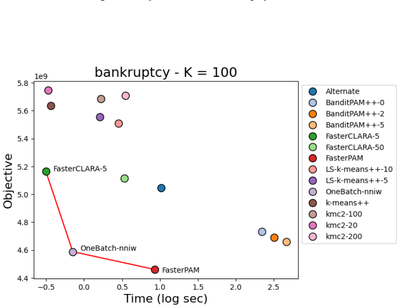
- On the paper's experiments, OneBatchPAM matches FasterPAM within about 2% objective while running roughly 7 times faster on small datasets, and it scales to datasets where FasterPAM cannot finish.
- The memory footprint drops from $O(n^2)$ to $O(n\log n)$ for stored dissimilarities, at the price of more memory than BanditPAM's $O(n)$.
- The nearest-neighbor importance-weighting variant (NNIW) gives the best objective in experiments and costs almost no extra time, since the required distances are already computed.
Reading between the lines
- Inference: The theorem's $\Delta$ is defined along FasterPAM's random trajectory; a dataset with near-duplicate points will have tiny $\Delta$, and the $1/\Delta^2$ factor can push the required batch above realistic values, so the practical regime is when objective gaps are not extremely small.
- Inference: The fixed-batch design suggests a streaming extension: after the initial $m\times n$ pass, each newly arrived point needs only $m$ distance computations, so the algorithm could maintain the same guarantee on a growing dataset without recomputing old distances.
- Inference: The paper's overfitting warning on imbalanced data points to a testable fix—make the batch adaptive by adding points whose nearest batch neighbor is atypically far, reusing all distances already computed, and compare the resulting objective on skewed datasets.
Signed reviews
Editorial analysis
A structured set of objections, weighed in public.
Referee Report
Summary. The paper introduces OneBatchPAM, a k-medoids local-search algorithm that estimates the PAM objective using a single random batch of size m drawn once from the dataset. The authors claim (Theorem 1) that m = O(log n) suffices, with probability at least 1 - delta, to reproduce the exact sequence of swaps of FasterPAM, yielding a time complexity of O((p + T)n log n) (Corollary 2). The empirical section compares OneBatchPAM variants against FasterPAM, BanditPAM++, FasterCLARA, k-means++ and related methods on small- and large-scale real datasets, reporting that OneBatchPAM (especially the NNIW variant) achieves objectives within about 2% of FasterPAM while running substantially faster.
Significance. If the main theorem were correct, the result would be significant: it would give a k-medoids local-search method with near-PAM quality at O(n log n) dissimilarity computations, improving on FasterPAM's O(n^2) and BanditPAM's O(T n log n). The empirical study is a genuine strength: the authors provide code, use public datasets, report standard deviations, and show consistent speedups with small objective degradation. The paper also honestly discusses limitations, including the dependence on the unknown margin Delta and the risk of overfitting on imbalanced data, which is commendable. However, the central theoretical guarantee is not proven as stated, and the authors' own limitation section concedes that in practice the algorithm does not return exactly the same medoid set as FasterPAM.
major comments (3)
- [Appendix B, proof of Theorem 1] The proof does not establish the claim that OneBatchPAM performs the same swaps as FasterPAM. For each data point i, Algorithm 2 (line 17) selects the medoid l* maximizing the empirical gain G_i^l, so the decision depends on the ranking of the k candidate swaps at that point. The proof bounds, for each rejected pair (x,x') in P_t, the probability that its empirical objective falls below the current empirical objective, and for the single selected pair (x_t,x'_t) the probability that its empirical objective rises above the current one. These are pairwise bounds; they do not control the event that a different improving pair at the same x_i has a larger empirical gain than the true best pair. The union bound in Eq. (25) covers only pairs in P_t (non-improving pairs) and the selected pair, not the improving-but-not-selected pairs whose empirical gains could be inflated by sampling error. Consequently, the event that OneBatchPAM picks a different medoid for the same data point, or a different data point, is not included in A, and the theorem is not proven. A repair would require a margin between the best and second-best candidate gains, or a weakened guarantee such as high-probability closeness of the objective value.
- [Discussion and Limitations, 'Minimum sample size of OneBatchPAM derived in Theorem 1'] The paper's own limitation paragraph states that if two objectives are close, OneBatchPAM 'may estimate that adding x to the set of medoids instead of x′ is more efficient while FasterPAM may do the opposite,' and that in experiments OneBatchPAM 'provides close objectives compared to FasterPAM (around 2% error) but not exactly the same.' This directly contradicts the exact same-medoid conclusion of Theorem 1 and indicates that the theorem's guarantee is not achieved by the practical algorithm with the heuristic batch size m = 100 log(kn). The authors should either revise Theorem 1 to state a weaker, defensible claim (e.g., high-probability approximation of the objective) or provide a proof that the exact-swap event holds under the stated sample-size condition.
- [Corollary 2 and complexity statement] Corollary 2 asserts time complexity O((p + T)n log(n)) from the logarithmic batch size, but the bound in Theorem 1 is m ≥ (4D²/Δ²) log(2Tn/δ), where Δ is an instance-dependent margin that can be arbitrarily small. Thus the logarithmic dependence on n comes with a constant that is not uniform over instances and can be enormous when near-tie swaps exist. The paper acknowledges in the Discussion that the exact value of Eq. (4) 'may be disproportionate' and that in practice m is chosen heuristically proportional to log n. Given that, the clean complexity statement of Corollary 2 is not justified by the theorem as written; the conditional dependence on Δ should be stated explicitly in the corollary.
minor comments (5)
- [Appendix B, Eq. (11)] The derivation 'It can be noticed that m ≥ 2D²/Δ² log(1/δ̃)' from Eq. (7) is valid because 4 log(2Tn/δ) ≥ 2 log(2Tn²/δ) for T ≥ 1 and δ ∈ (0,1], but the algebra is not shown; writing the intervening inequality would prevent reader confusion.
- [Theorem 1 statement] The definition of Δ uses an absolute value and includes pairs with equal objectives, so Δ can be zero; the proof requires Δ > 0. This assumption should be stated explicitly in the theorem statement rather than only implicitly in the Discussion.
- [Algorithm 2, line 19] The condition 'if G_i > 0' compares the empirical gain to zero, whereas FasterPAM's true improvement condition is L(M_t) > L(M_t \ {x} ∪ {x′}); the algorithm description should clarify how the empirical quantities relate to the true objective and whether strict vs. non-strict improvement is used.
- [Discussion and Limitations] There is a typo: 'FatserPAM' should be 'FasterPAM'.
- [Table 1] The entry for FasterCLARA is difficult to read: 'I (p + T )k2 + pkn' lacks formatting clarity, and the k-means++ entry lists 'log(k)' as the approximation factor without indicating the usual O(log k)-approximation notation.
Circularity Check
No significant circularity: the batch-size theorem is a concentration bound with data-dependent constants, not an input fitted as a prediction; the proof gap about swap ranking is a soundness issue, not circularity.
full rationale
The derivation is self-contained. Theorem 1 (main text and Appendix B) bounds the probability that OneBatchPAM's empirical objective, computed on a uniformly drawn batch of size m, deviates from the true k-medoids objective by more than a Hoeffding tolerance C, and then uses the margin Delta to ensure that estimated objective comparisons preserve the order of every swap pair evaluated by FasterPAM. The constants D and Delta are properties of the dataset and of the reference FasterPAM trajectory, not fitted parameters, and Delta is not estimated from the batch nor tuned to make the guarantee hold. The theorem is therefore a conditional concentration bound rather than a restatement of its conclusion. The one self-citation (de Mathelin et al. 2021) appears only as an application example in the introduction and is not load-bearing. The practical batch size m = 100 log(kn) is explicitly presented as a heuristic: the paper states, 'In practice, we do not estimate the ratio D/Delta to set the sample size, but instead choose a value proportional to log(n)', so the experiments are not using a fitted constant disguised as a prediction. The discussion and limitations section honestly concedes that a small Delta can force a large batch and that the exact formula may be disproportionate. A separate correctness caveat should be flagged in Appendix B: the proof bounds probabilities that rejected pairs are estimated as improving and that the FasterPAM-selected pair is estimated as non-improving, but it does not bound the probability that OneBatchPAM ranks a different improving swap above the FasterPAM-selected swap; event A in Eq. (25) does not cover that failure mode. This is a soundness gap in the proof of Theorem 1, not a circular reduction, and it does not raise the circularity score beyond the negligible self-citation level.
Assumptions & free parameters
free parameters (1)
- batch size m =
100 log(k n) in experiments
assumptions (4)
- standard math Hoeffding inequality applies to each batch objective estimate
- domain assumption Dissimilarities are bounded by D
- ad hoc to paper Minimum objective gap Delta is strictly positive
- domain assumption Uniform random sampling from Xn
Cite this review
Pith. "Pith review of OneBatchPAM: A Fast and Frugal K-Medoids Algorithm." pith.science (2026). https://pith.science/paper/E72JCTDH
@misc{pith2026250119285,
  author       = {Pith},
  title        = {Pith review of: OneBatchPAM: A Fast and Frugal K-Medoids Algorithm},
  year         = {2026},
  howpublished = {\url{https://pith.science/paper/E72JCTDH}},
  note         = {Machine review of arXiv:2501.19285}
}
read the original abstract
This paper proposes a novel k-medoids approximation algorithm to handle large-scale datasets with reasonable computational time and memory complexity. We develop a local-search algorithm that iteratively improves the medoid selection based on the estimation of the k-medoids objective. A single batch of size m << n provides the estimation, which reduces the required memory size and the number of pairwise dissimilarities computations to O(mn), instead of O(n^2) compared to most k-medoids baselines. We obtain theoretical results highlighting that a batch of size m = O(log(n)) is sufficient to guarantee, with strong probability, the same performance as the original local-search algorithm. Multiple experiments conducted on real datasets of various sizes and dimensions show that our algorithm provides similar performances as state-of-the-art methods such as FasterPAM and BanditPAM++ with a drastically reduced running time.
Figures


Figures from the paper (28 more)




Reference graph
Works this paper leans on
-
[1]
, " * write output.state after.block = add.period write newline
ENTRY address archivePrefix author booktitle chapter edition editor eid eprint howpublished institution isbn journal key month note number organization pages publisher school series title type volume year label extra.label sort.label short.list INTEGERS output.state before.all mid.sentence after.sentence after.block FUNCTION init.state.consts #0 'before.a...
-
[2]
write newline
" write newline "" before.all 'output.state := FUNCTION n.dashify 't := "" t empty not t #1 #1 substring "-" = t #1 #2 substring "--" = not "--" * t #2 global.max substring 't := t #1 #1 substring "-" = "-" * t #2 global.max substring 't := while if t #1 #1 substring * t #2 global.max substring 't := if while FUNCTION word.in bbl.in capitalize " " * FUNCT...
-
[3]
Arthur, D.; Vassilvitskii, S.; et al. 2007. k-means++: The advantages of careful seeding. In Soda, volume 7, 1027--1035
work page 2007
-
[4]
Arya, V.; Garg, N.; Khandekar, R.; Meyerson, A.; Munagala, K.; and Pandit, V. 2001. Local search heuristic for k-median and facility location problems. In Proceedings of the thirty-third annual ACM symposium on Theory of computing, 21--29
work page 2001
-
[5]
Bachem, O.; Lucic, M.; Hassani, S. H.; and Krause, A. 2016. Approximate k-means++ in sublinear time. In Proceedings of the AAAI conference on artificial intelligence, volume 30
work page 2016
-
[6]
Bachem, O.; Lucic, M.; and Krause, A. 2018. Scalable k-means clustering via lightweight coresets. In Proceedings of the 24th ACM SIGKDD International Conference on Knowledge Discovery & Data Mining, 1119--1127
work page 2018
-
[7]
Beretta, L.; Cohen-Addad, V.; Lattanzi, S.; and Parotsidis, N. 2024. Multi-Swap k-Means++. Advances in Neural Information Processing Systems, 36
work page 2024
-
[8]
Bhat, A. 2014. K-medoids clustering using partitioning around medoids for performing face recognition. International Journal of Soft Computing, Mathematics and Control, 3(3): 1--12
work page 2014
Show all 53 references
-
[9]
S.; Krauthgamer, R.; Schwiegelshohn, C.; Toftrup, M
Braverman, V.; Cohen-Addad, V.; Jiang, H.-C. S.; Krauthgamer, R.; Schwiegelshohn, C.; Toftrup, M. B.; and Wu, X. 2022. The power of uniform sampling for coresets. In 2022 IEEE 63rd Annual Symposium on Foundations of Computer Science (FOCS), 462--473. IEEE
2022
-
[10]
Byrka, J.; Pensyl, T.; Rybicki, B.; Srinivasan, A.; and Trinh, K. 2017. An improved approximation for k-median and positive correlation in budgeted optimization. ACM Transactions on Algorithms (TALG), 13(2): 1--31
2017
-
[11]
Charikar, M.; Guha, S.; Tardos, \'E .; and Shmoys, D. B. 1999. A constant-factor approximation algorithm for the k-median problem. In Proceedings of the thirty-first annual ACM symposium on Theory of computing, 1--10
1999
-
[12]
Charikar, M.; Henzinger, M.; Hu, L.; V \"o tsch, M.; and Waingarten, E. 2023. Simple, scalable and effective clustering via one-dimensional projections. Advances in Neural Information Processing Systems, 36: 64618--64649
2023
-
[13]
Chen, K. 2009. On coresets for k-median and k-means clustering in metric and euclidean spaces and their applications. SIAM Journal on Computing, 39(3): 923--947
2009
-
[14]
Chrobak, M.; Kenyon, C.; and Young, N. 2006. The reverse greedy algorithm for the metric k-median problem. Information Processing Letters, 97(2): 68--72
2006
-
[15]
G.; Saulpic, D.; and Schwiegelshohn, C
Cohen-Addad, V.; Larsen, K. G.; Saulpic, D.; and Schwiegelshohn, C. 2022. Towards optimal lower bounds for k-median and k-means coresets. In Proceedings of the 54th Annual ACM SIGACT Symposium on Theory of Computing, 1038--1051
2022
-
[16]
Cohen-Addad, V.; Lattanzi, S.; Norouzi-Fard, A.; Sohler, C.; and Svensson, O. 2020. Fast and accurate k -means++ via rejection sampling. Advances in Neural Information Processing Systems, 33: 16235--16245
2020
-
[17]
Cohen-Addad, V.; Saulpic, D.; and Schwiegelshohn, C. 2021 a . Improved coresets and sublinear algorithms for power means in euclidean spaces. Advances in Neural Information Processing Systems, 34: 21085--21098
2021
-
[18]
Cohen-Addad, V.; Saulpic, D.; and Schwiegelshohn, C. 2021 b . A new coreset framework for clustering. In Proceedings of the 53rd Annual ACM SIGACT Symposium on Theory of Computing, 169--182
2021
-
[19]
Czumaj, A.; and Sohler, C. 2007. Sublinear-time approximation algorithms for clustering via random sampling. Random Structures & Algorithms, 30(1-2): 226--256
2007
-
[20]
de Mathelin, A.; Deheeger, F.; MOUGEOT, M.; and Vayatis, N. 2021. Discrepancy-Based Active Learning for Domain Adaptation. In International Conference on Learning Representations
2021
-
[21]
Dohan, D.; Karp, S.; and Matejek, B. 2015. K-median algorithms: theory in practice. Princeton University
2015
-
[22]
Dua, D.; and Graff, C. 2017. UCI Machine Learning Repository
2017
-
[23]
Feldman, D. 2020. Core-sets: Updated survey. Sampling techniques for supervised or unsupervised tasks, 23--44
2020
-
[24]
Feldman, D.; and Langberg, M. 2011. A unified framework for approximating and clustering data. In Proceedings of the forty-third annual ACM symposium on Theory of computing, 569--578
2011
-
[25]
Guha, S.; and Mishra, N. 2016. Clustering data streams. In Data stream management: processing high-speed data streams, 169--187. Springer
2016
-
[26]
Har-Peled, S.; and Mazumdar, S. 2004. On coresets for k-means and k-median clustering. In Proceedings of the thirty-sixth annual ACM symposium on Theory of computing, 291--300
2004
-
[27]
Huang, J.; Feng, Q.; Huang, Z.; Xu, J.; and Wang, J. 2024. Linear Time Algorithms for k-means with Multi-Swap Local Search. Advances in Neural Information Processing Systems, 36
2024
-
[28]
H.-C.; and Lou, J
Huang, L.; Jiang, S. H.-C.; and Lou, J. 2023. The power of uniform sampling for k-median. In International Conference on Machine Learning, 13933--13956. PMLR
2023
-
[29]
Jaiswal, R.; and Kumar, A. 2024. Universal Weak Coreset. In Proceedings of the AAAI Conference on Artificial Intelligence, volume 38, 12782--12789
2024
-
[30]
Kariv, S.; and Hakimi, O. 1979. An algorithmic approach to network location problems. II: the p-medians. SIAM J. Appl. Math, 37(3): 539
1979
-
[31]
Kaufman, L. 1986. Clustering large data sets. Pattern recognition in practice, 425--437
1986
-
[32]
Kaufman, L. 1990. Partitioning around medoids (program pam). Finding groups in data, 344: 68--125
1990
-
[33]
Kaufman, L.; and Rousseeuw, P. J. 1987. Clustering by means of Medoids. Statistical data analysis based on the L1--norm and related methods, edited by Y. Dodge
1987
-
[34]
Kaufman, L.; and Rousseeuw, P. J. 2008. Clustering large applications (Program CLARA). Finding groups in data: an introduction to cluster analysis, 126--63
2008
-
[35]
Kaushal, V.; Iyer, R.; Kothawade, S.; Mahadev, R.; Doctor, K.; and Ramakrishnan, G. 2019. Learning from less data: A unified data subset selection and active learning framework for computer vision. In 2019 IEEE Winter Conference on Applications of Computer Vision (WACV), 1289-...
2019
-
[36]
Krizhevsky, A.; Hinton, G.; et al. 2009. Learning multiple layers of features from tiny images
2009
-
[37]
Lattanzi, S.; and Sohler, C. 2019. A better k-means++ algorithm via local search. In International Conference on Machine Learning, 3662--3671. PMLR
2019
-
[38]
LeCun, Y.; Cortes, C.; and Burges, C. J. 1994. The MNIST databaseof handwritten digits
1994
-
[39]
Li, S.; and Svensson, O. 2013. Approximating k-median via pseudo-approximation. In proceedings of the forty-fifth annual ACM symposium on theory of computing, 901--910
2013
-
[40]
Loog, M. 2012. Nearest neighbor-based importance weighting. In 2012 IEEE international workshop on machine learning for signal processing, 1--6. IEEE
2012
-
[41]
R.; and Plaxton, C
Mettu, R. R.; and Plaxton, C. G. 2004. Optimal time bounds for approximate clustering. Machine Learning, 56(1): 35--60
2004
-
[42]
Meyerson, A.; O'callaghan, L.; and Plotkin, S. 2004. A k-median algorithm with running time independent of data size. Machine Learning, 56(1): 61--87
2004
-
[43]
Mishra, N.; Oblinger, D.; and Pitt, L. 2001. Sublinear time approximate clustering. In SODA, volume 1, 439--447
2001
-
[44]
Park, H.-S.; and Jun, C.-H. 2009. A simple and fast algorithm for K-medoids clustering. Expert systems with applications, 36(2): 3336--3341
2009
-
[45]
Pelleg, D.; and Moore, A. 1999. Accelerating exact k-means algorithms with geometric reasoning. In Proceedings of the fifth ACM SIGKDD international conference on Knowledge discovery and data mining, 277--281
1999
-
[46]
Ren, J.; Hua, K.; and Cao, Y. 2022. Global optimal k-medoids clustering of one million samples. Advances in Neural Information Processing Systems, 35: 982--994
2022
-
[47]
Schmidt, M.; Schwiegelshohn, C.; and Sohler, C. 2020. Fair coresets and streaming algorithms for fair k-means. In Approximation and Online Algorithms: 17th International Workshop, WAOA 2019, Munich, Germany, September 12--13, 2019, Revised Selected Papers 17, 232--251. Springer
2020
-
[48]
Schubert, E.; and Lenssen, L. 2022. Fast k-medoids Clustering in Rust and Python. Journal of Open Source Software, 7(75): 4183
2022
-
[49]
Schubert, E.; and Rousseeuw, P. J. 2021. Fast and eager k-medoids clustering: O (k) runtime improvement of the PAM, CLARA, and CLARANS algorithms. Information Systems, 101: 101804
2021
-
[50]
Thorup, M. 2005. Quick k-median, k-center, and facility location for sparse graphs. SIAM Journal on Computing, 34(2): 405--432
2005
-
[51]
Tiwari, M.; Kang, R.; Lee, D.; Thrun, S.; Shomorony, I.; and Zhang, M. J. 2023. BanditPAM++: Faster k -medoids Clustering. Advances in Neural Information Processing Systems, 36: 73371--73382
2023
-
[52]
J.; Mayclin, J.; Thrun, S.; Piech, C.; and Shomorony, I
Tiwari, M.; Zhang, M. J.; Mayclin, J.; Thrun, S.; Piech, C.; and Shomorony, I. 2020. Banditpam: Almost linear time k-medoids clustering via multi-armed bandits. Advances in Neural Information Processing Systems, 33: 10211--10222
2020
-
[53]
Wei, K.; Iyer, R.; and Bilmes, J. 2015. Submodularity in data subset selection and active learning. In International conference on machine learning, 1954--1963. PMLR
2015
Reviewed August 9, 2026 · model on record in the stance chip above.
Discussion (0). Continue with ORCID to comment.