pith. sign in

arxiv: 2504.10435 · v4 · submitted 2025-04-14 · 🧮 math.NA · cs.NA· physics.comp-ph

What metric to optimize for suppressing instability in a Vlasov-Poisson system?

Pith reviewed 2026-05-22 19:39 UTC · model grok-4.3

classification 🧮 math.NA cs.NAphysics.comp-ph
keywords Vlasov-Poisson systemplasma stabilizationPDE-constrained optimizationobjective functionsinstability suppressiondispersion relationgradient-based optimization
0
0 comments X

The pith

Time-integrated objective functions create more convex-like landscapes that favor gradient-based optimization for suppressing instabilities in the Vlasov-Poisson system.

A machine-rendered reading of the paper's core claim, the machinery that carries it, and where it could break.

The paper studies how to select objective functions when using PDE-constrained optimization to find external electric fields that stabilize a simplified Vlasov-Poisson plasma model. Dispersion relation analysis identifies parameter values that remove unstable modes and serve as strong starting points for the optimizer. Numerical tests then compare several candidate objectives and find that those which accumulate information across time produce smoother, more convex optimization surfaces. These surfaces make gradient methods more reliable than objectives that rely only on instantaneous states. The results are meant to inform objective design for control problems in kinetic plasma models.

Core claim

Analysis of the dispersion relation for the Vlasov-Poisson system yields parameter configurations that eliminate unstable modes and lie close to the global optimum, serving as effective initial guesses. Numerical experiments comparing objective functions show that different choices lead to similar stabilizing configurations, yet objectives that incorporate time-integrated information exhibit more convex-like landscapes and are therefore more favorable for gradient-based optimization methods.

What carries the argument

PDE-constrained optimization of external electric fields, with objective functions evaluated through their resulting optimization landscapes and informed by dispersion relation analysis for initialization.

If this is right

  • Dispersion analysis supplies initial guesses that lie close to the global optimum.
  • Different objective functions converge to similar stabilizing parameter sets.
  • Time-integrated objectives generate smoother landscapes that improve the performance of gradient descent.
  • These landscape properties can guide the design of objective functions for optimization-based plasma control.

Where Pith is reading between the lines

These are editorial extensions of the paper, not claims the author makes directly.

  • The same dispersion-based initialization strategy could be tested on other linear kinetic models before moving to nonlinear regimes.
  • Precomputed spectral information might reduce the cost of real-time control loops if the underlying dynamics remain close to the linear regime.
  • Extension to three-dimensional or multi-species plasmas would clarify whether the convexity benefit persists when the dispersion relation becomes more intricate.

Load-bearing premise

The optimization landscapes measured on the simplified Vlasov-Poisson system are representative of those that appear in the more complex kinetic plasma models used for actual fusion control.

What would settle it

A single optimization run on a higher-dimensional or nonlinear kinetic model in which a time-integrated objective produces a markedly non-convex landscape with many poor local minima would contradict the claimed advantage.

Figures
Figures reproduced from arXiv: 2504.10435 by Leonardo Zepeda-N\'u\~nez, Martin Guerra, Qin Li, Yukun Yue.

Figure 1
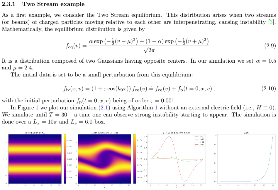
Figure 1. Figure 1: Simulation of (2.1) with H ≡ 0 for the Two Stream equilibrium. From left to right we have feq(v), f(T = 30, x, v), Ef (t, x) and Ef (t). 2.3.2 Bump-on-Tail example The Bump-on-Tail equilibrium is another steady state that is heavily investigated. This distribution appears when a small group of fast-moving electrons (a “bump”) is superimposed on the tail of the background electron velocity distribution and … view at source ↗
Figure 2
Figure 2. Figure 2: Simulation of (2.1) with H ≡ 0 for the Bump-on-Tail equilibrium. From left to right we have feq(v), f(T = 40, x, v), Ef (t, x) and Ef (t). 3 Dispersion relation and linear stability analysis Examining the dispersion relation is a classical approach to investigating the stability properties of dynamical systems [39]. Mathematically, this involves linearizing the system around a desired equilibrium state and… view at source ↗
Figure 3
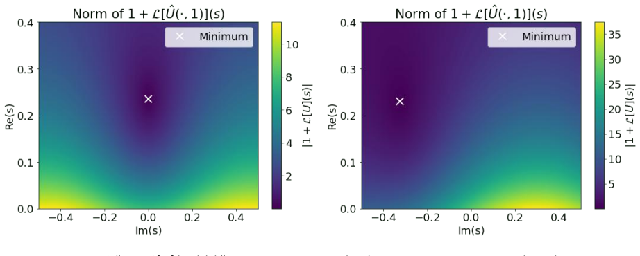
Figure 3. Figure 3: Norm of ∥1 + L[U](·, 1)(s)∥: the Two Stream (left) and the Bump-on-Tail (right) examples. In Two Stream, the minimum occurs at s0 = 0.236 + 0i with ∥1 + L[U](·, 1)(s0)∥ = 9.564044 × 10⁻⁴ . In Bump￾on-Tail, the minimum occurs at s0 = 0.230 − 0.324i with ∥1 + L[U](·, 1)(s0)∥ = 3.756278 × 10⁻³ . 4 Landscape analysis of the objective function In this section, we examine the landscape of the objective function.… view at source ↗
Figure 4
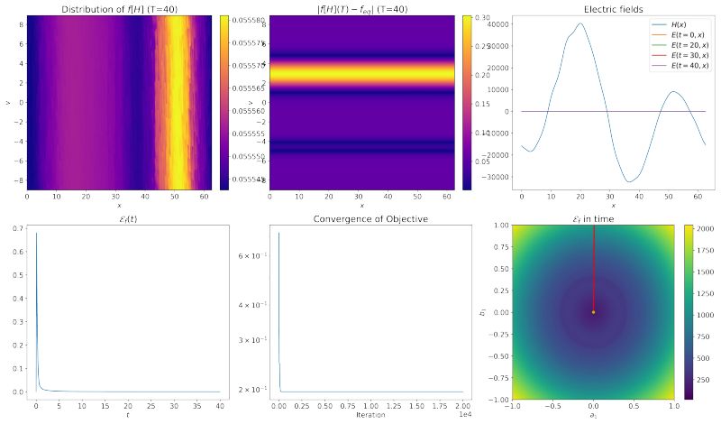
Figure 4. Figure 4: Simulation of (2.1) for the Two Stream equilibrium up to T = 30 (top) and Bump-on-Tail equilibrium up to T = 40 (bottom). In each row, from left to right: feq(v), f(T, x, v) (for H ≡ 0), f(T, x, v) (for H obtained from Example 3.1) and Ef (t) (for H ≡ 0 and H obtained from Example 3.1) [PITH_FULL_IMAGE:figures/full_fig_p012_4.png] view at source ↗
Figure 5
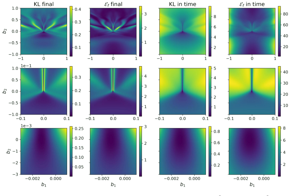
Figure 5. Figure 5: Landscape of the Two Stream instability on the domain [ [PITH_FULL_IMAGE:figures/full_fig_p012_5.png] view at source ↗
Figure 6
Figure 6. Figure 6: Landscape of the Two Stream instability with on the domain [ [PITH_FULL_IMAGE:figures/full_fig_p013_6.png] view at source ↗
Figure 7
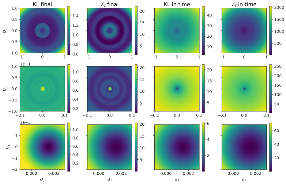
Figure 7. Figure 7: Landscape of the Bump-on-Tail instability on the domain [ [PITH_FULL_IMAGE:figures/full_fig_p014_7.png] view at source ↗
Figure 8
Figure 8. Figure 8: Landscape of the Bump-on-Tail instability with on the domain [ [PITH_FULL_IMAGE:figures/full_fig_p015_8.png] view at source ↗
Figure 9
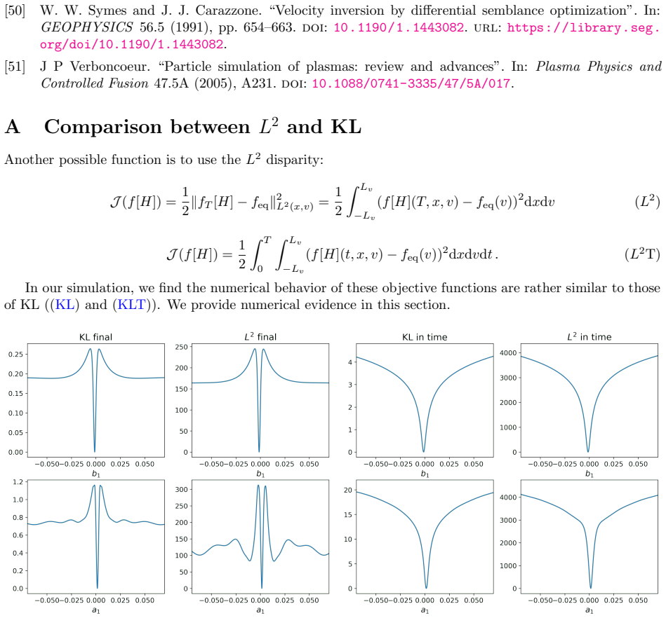
Figure 9. Figure 9: Landscape of Two Stream instability for b1 for (4.1)(top) and Bump-on-Tail instability for a1 for (4.3)(bottom) on the domain [0.07, 0.07] of the objectives (KL)(left), (L 2 )(center-left), (KLT)(center￾right) and (L 2T)(right). In [PITH_FULL_IMAGE:figures/full_fig_p022_9.png] view at source ↗
Figure 10
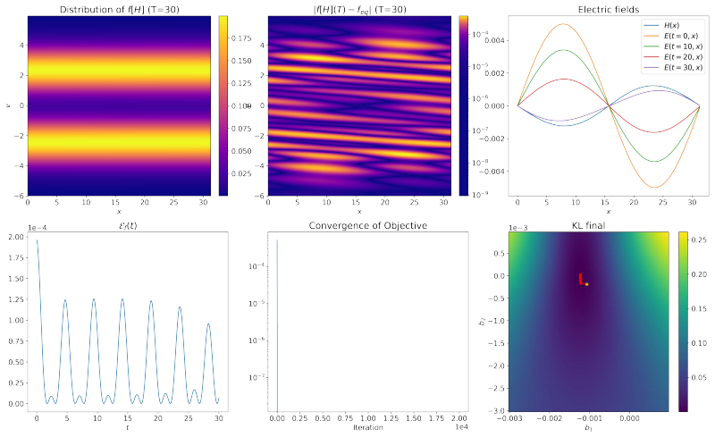
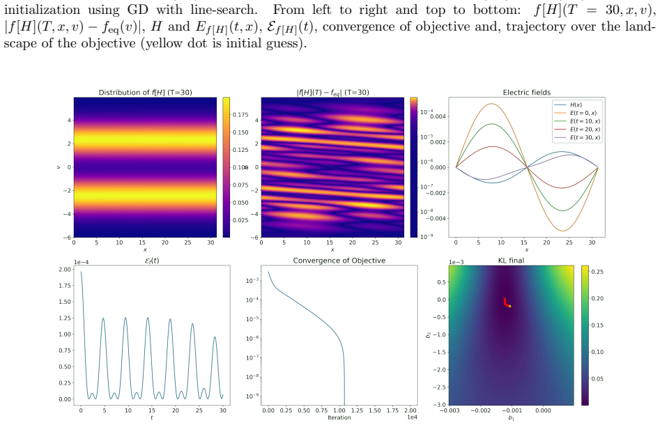
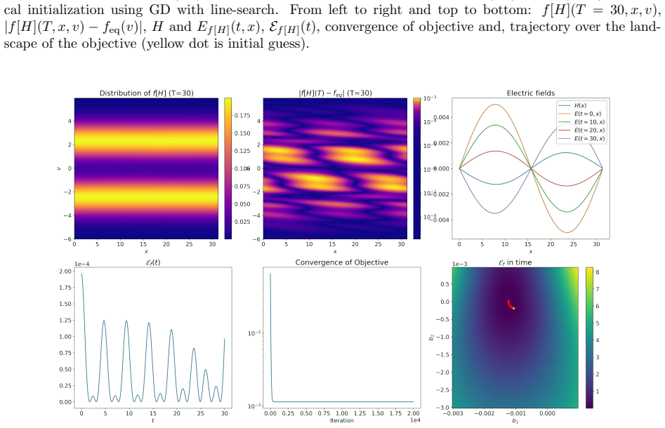
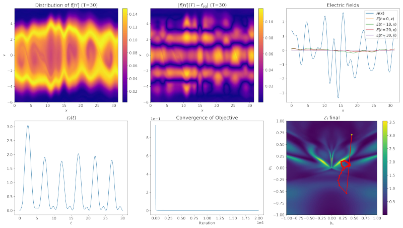
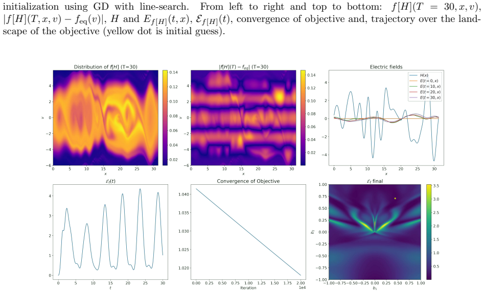
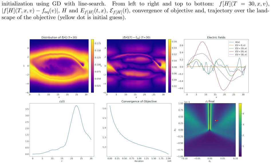
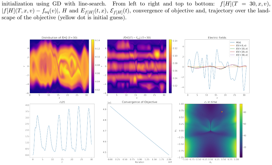
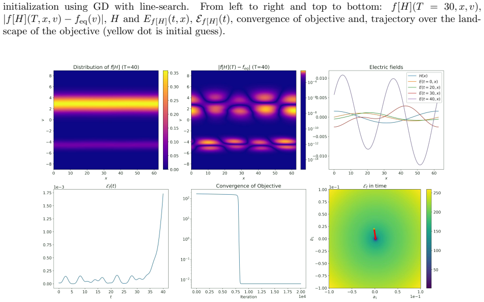
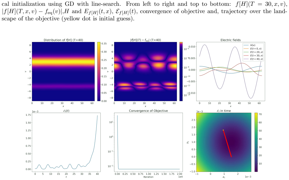
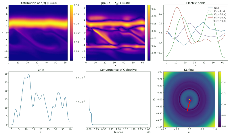
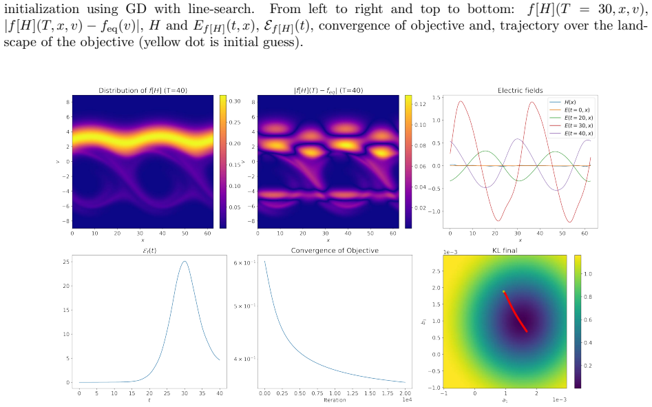
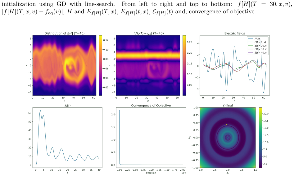
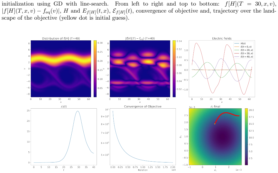
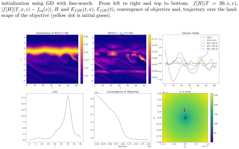
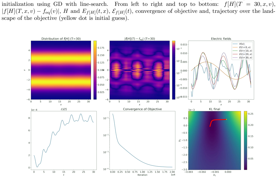
Figure 10. Figure 10: Simulation of (2.1) with under-parametrized H obtained from (2.6) using (KL) with far initialization using GD with line-search. From left to right and top to bottom: f[H](T = 30, x, v), |f[H](T, x, v) − feq(v)|, H and Ef[H](t, x), Ef[H](t), convergence of objective and, trajectory over the land￾scape of the objective (yellow dot is initial guess) [PITH_FULL_IMAGE:figures/full_fig_p023_10.png] view at source ↗
Figure 11
Figure 11. Figure 11: Simulation of (2.1) with under-parametrized H obtained from (2.6) using (KL) with far ini￾tialization using GD with constant stepsize. From left to right and top to bottom: f[H](T = 30, x, v), |f[H](T, x, v) − feq(v)|, H and Ef[H](t, x), Ef[H](t), convergence of objective and, trajectory over the land￾scape of the objective (yellow dot is initial guess). 23 [PITH_FULL_IMAGE:figures/full_fig_p023_11.png] view at source ↗
Figure 12
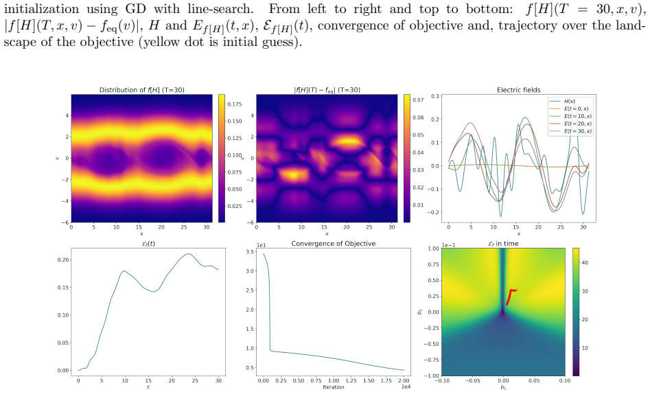
Figure 12. Figure 12: Simulation of (2.1) with under-parametrized H obtained from (2.6) using (KL) with near initialization using GD with line-search. From left to right and top to bottom: f[H](T = 30, x, v), |f[H](T, x, v) − feq(v)|, H and Ef[H](t, x), Ef[H](t), convergence of objective and, trajectory over the land￾scape of the objective (yellow dot is initial guess) [PITH_FULL_IMAGE:figures/full_fig_p024_12.png] view at source ↗
Figure 13
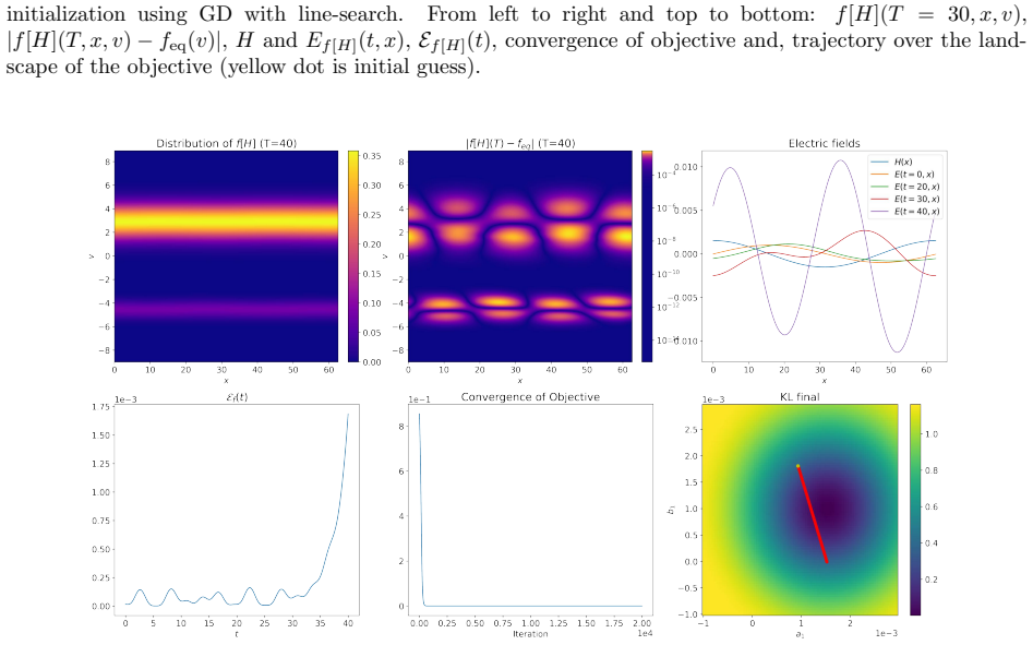
Figure 13. Figure 13: Simulation of (2.1) with under-parametrized H obtained from (2.6) using (KL) with near ini￾tialization using GD with constant stepsize. From left to right and top to bottom: f[H](T = 30, x, v), |f[H](T, x, v) − feq(v)|, H and Ef[H](t, x), Ef[H](t), convergence of objective and, trajectory over the land￾scape of the objective (yellow dot is initial guess). 24 [PITH_FULL_IMAGE:figures/full_fig_p024_13.png] view at source ↗
Figure 14
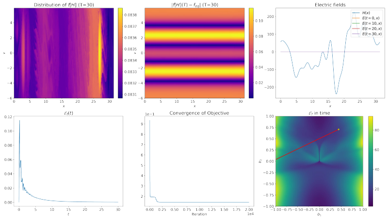
Figure 14. Figure 14: Simulation of (2.1) with under-parametrized H obtained from (2.6) using (KL) with local initialization using GD with line-search. From left to right and top to bottom: f[H](T = 30, x, v), |f[H](T, x, v) − feq(v)|, H and Ef[H](t, x), Ef[H](t), convergence of objective and, trajectory over the land￾scape of the objective (yellow dot is initial guess) [PITH_FULL_IMAGE:figures/full_fig_p025_14.png] view at source ↗
Figure 15
Figure 15. Figure 15: Simulation of (2.1) with under-parametrized H obtained from (2.6) using (KL) with local ini￾tialization using GD with constant stepsize. From left to right and top to bottom: f[H](T = 30, x, v), |f[H](T, x, v) − feq(v)|, H and Ef[H](t, x), Ef[H](t), convergence of objective and, trajectory over the land￾scape of the objective (yellow dot is initial guess). 25 [PITH_FULL_IMAGE:figures/full_fig_p025_15.png] view at source ↗
Figure 16
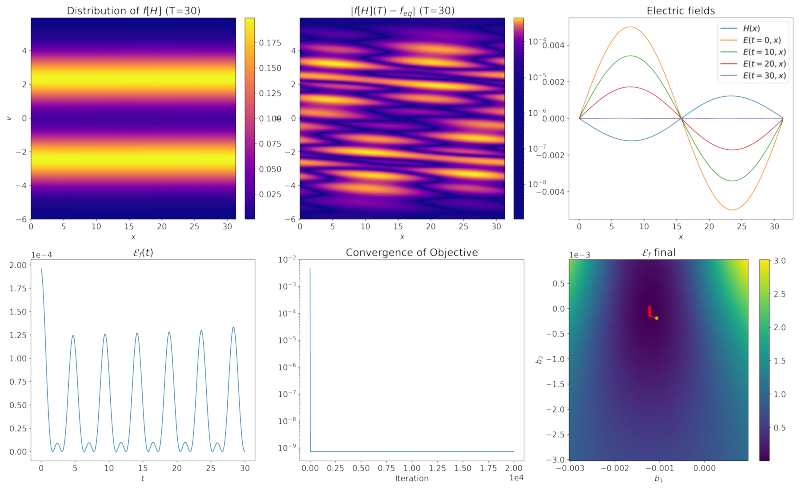
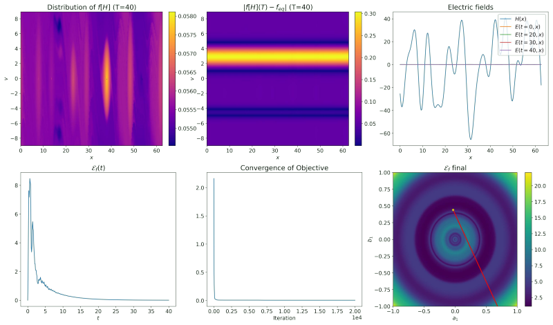
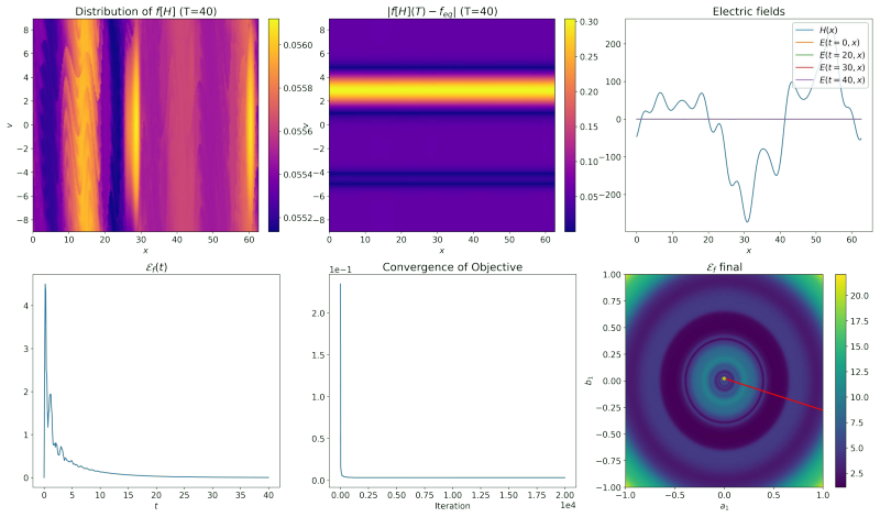
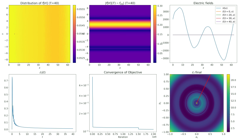
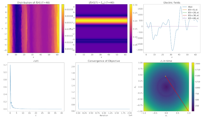
Figure 16. Figure 16: Simulation of (2.1) with under-parametrized H obtained from (2.6) using (EE) with far initialization using GD with line-search. From left to right and top to bottom: f[H](T = 30, x, v), |f[H](T, x, v) − feq(v)|, H and Ef[H](t, x), Ef[H](t), convergence of objective and, trajectory over the land￾scape of the objective (yellow dot is initial guess) [PITH_FULL_IMAGE:figures/full_fig_p026_16.png] view at source ↗
Figure 17
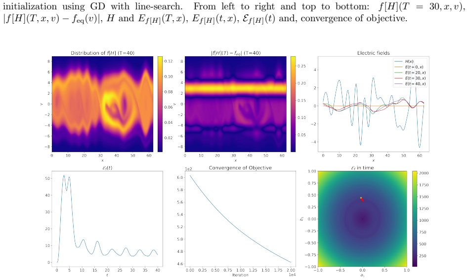
Figure 17. Figure 17: Simulation of (2.1) with under-parametrized H obtained from (2.6) using (EE) with far ini￾tialization using GD with constant stepsize. From left to right and top to bottom: f[H](T = 30, x, v), |f[H](T, x, v) − feq(v)|, H and Ef[H](T, x), Ef[H](t, x), Ef[H](t) and, convergence of objective. 26 [PITH_FULL_IMAGE:figures/full_fig_p026_17.png] view at source ↗
Figure 18
Figure 18. Figure 18: Simulation of (2.1) with under-parametrized H obtained from (2.6) using (EE) with near initialization using GD with line-search. From left to right and top to bottom: f[H](T = 30, x, v), |f[H](T, x, v) − feq(v)|, H and Ef[H](t, x), Ef[H](t), convergence of objective and, trajectory over the land￾scape of the objective (yellow dot is initial guess) [PITH_FULL_IMAGE:figures/full_fig_p027_18.png] view at source ↗
Figure 19
Figure 19. Figure 19: Simulation of (2.1) using (EE) with under-parametrized H obtained from (2.6) with near ini￾tialization using GD with constant stepsize. From left to right and top to bottom: f[H](T = 30, x, v), |f[H](T, x, v) − feq(v)|, H and Ef[H](t, x), Ef[H](t), convergence of objective and, trajectory over the land￾scape of the objective (yellow dot is initial guess). 27 [PITH_FULL_IMAGE:figures/full_fig_p027_19.png] view at source ↗
Figure 20
Figure 20. Figure 20: Simulation of (2.1) with under-parametrized H obtained from (2.6) using (EE) with local initialization using GD with line-search. From left to right and top to bottom: f[H](T = 30, x, v), |f[H](T, x, v) − feq(v)|, H and Ef[H](t, x), Ef[H](t), convergence of objective and, trajectory over the land￾scape of the objective (yellow dot is initial guess) [PITH_FULL_IMAGE:figures/full_fig_p028_20.png] view at source ↗
Figure 21
Figure 21. Figure 21: Simulation of (2.1) using (EE) with under-parametrized H obtained from (2.6) with local ini￾tialization using GD with constant stepsize. From left to right and top to bottom: f[H](T = 30, x, v), |f[H](T, x, v) − feq(v)|, H and Ef[H](t, x), Ef[H](t), convergence of objective and, trajectory over the land￾scape of the objective (yellow dot is initial guess). 28 [PITH_FULL_IMAGE:figures/full_fig_p028_21.png] view at source ↗
Figure 22
Figure 22. Figure 22: Simulation of (2.1) with under-parametrized H obtained from (2.6) using (EET) with far initialization using GD with line-search. From left to right and top to bottom: f[H](T = 30, x, v), |f[H](T, x, v) − feq(v)|, H and Ef[H](t, x), Ef[H](t), convergence of objective and, trajectory over the land￾scape of the objective (yellow dot is initial guess) [PITH_FULL_IMAGE:figures/full_fig_p029_22.png] view at source ↗
Figure 23
Figure 23. Figure 23: Simulation of (2.1) with under-parametrized H obtained from (2.6) using (EET) with far ini￾tialization using GD with constant stepsize. From left to right and top to bottom: f[H](T = 30, x, v), |f[H](T, x, v) − feq(v)|, H and Ef[H](T, x), Ef[H](t, x), Ef[H](t) and, convergence of objective. 29 [PITH_FULL_IMAGE:figures/full_fig_p029_23.png] view at source ↗
Figure 24
Figure 24. Figure 24: Simulation of (2.1) with under-parametrized H obtained from (2.6) using (EET) with near initialization using GD with line-search. From left to right and top to bottom: f[H](T = 30, x, v), |f[H](T, x, v) − feq(v)|, H and Ef[H](t, x), Ef[H](t), convergence of objective and, trajectory over the land￾scape of the objective (yellow dot is initial guess) [PITH_FULL_IMAGE:figures/full_fig_p030_24.png] view at source ↗
Figure 25
Figure 25. Figure 25: Simulation of (2.1) using (EET) with under-parametrized H obtained from (2.6) with near ini￾tialization using GD with constant stepsize. From left to right and top to bottom: f[H](T = 30, x, v), |f[H](T, x, v) − feq(v)|, H and Ef[H](t, x), Ef[H](t), convergence of objective and, trajectory over the land￾scape of the objective (yellow dot is initial guess). 30 [PITH_FULL_IMAGE:figures/full_fig_p030_25.png] view at source ↗
Figure 26
Figure 26. Figure 26: Simulation of (2.1) with under-parametrized H obtained from (2.6) using (EET) with lo￾cal initialization using GD with line-search. From left to right and top to bottom: f[H](T = 30, x, v), |f[H](T, x, v) − feq(v)|, H and Ef[H](t, x), Ef[H](t), convergence of objective and, trajectory over the land￾scape of the objective (yellow dot is initial guess) [PITH_FULL_IMAGE:figures/full_fig_p031_26.png] view at source ↗
Figure 27
Figure 27. Figure 27: Simulation of (2.1) using (EET) with under-parametrized H obtained from (2.6) with local ini￾tialization using GD with constant stepsize. From left to right and top to bottom: f[H](T = 30, x, v), |f[H](T, x, v) − feq(v)|, H and Ef[H](t, x), Ef[H](t), convergence of objective and, trajectory over the land￾scape of the objective (yellow dot is initial guess). 31 [PITH_FULL_IMAGE:figures/full_fig_p031_27.png] view at source ↗
Figure 28
Figure 28. Figure 28: Simulation of (2.1) with over-parametrized H obtained from (2.6) using (KL) with far initialization using GD with line-search. From left to right and top to bottom: f[H](T = 30, x, v), |f[H](T, x, v)−feq(v)|, H and Ef[H](t, x), Ef[H](t), convergence of objective and, trajectory over the landscape of the objective (yellow dot is initial guess) [PITH_FULL_IMAGE:figures/full_fig_p032_28.png] view at source ↗
Figure 29
Figure 29. Figure 29: Simulation of (2.1) with over-parametrized H obtained from (2.6) using (KL) with far initialization using GD with constant stepsize. From left to right and top to bottom: f[H](T = 30, x, v), |f[H](T, x, v) − feq(v)|, H and Ef[H](t, x), Ef[H](t), convergence of objective and, trajectory over the landscape of the objective (yellow dot is initial guess). 32 [PITH_FULL_IMAGE:figures/full_fig_p032_29.png] view at source ↗
Figure 30
Figure 30. Figure 30: Simulation of (2.1) with over-parametrized H obtained from (2.6) using (KL) with near initialization using GD with line-search. From left to right and top to bottom: f[H](T = 30, x, v), |f[H](T, x, v) − feq(v)|, H and Ef[H](t, x), Ef[H](t), convergence of objective and, trajectory over the land￾scape of the objective (yellow dot is initial guess) [PITH_FULL_IMAGE:figures/full_fig_p033_30.png] view at source ↗
Figure 31
Figure 31. Figure 31: Simulation of (2.1) with over-parametrized H obtained from (2.6) using (KL) with near ini￾tialization using GD with constant stepsize. From left to right and top to bottom: f[H](T = 30, x, v), |f[H](T, x, v) − feq(v)|, H and Ef[H](t, x), Ef[H](t), convergence of objective and, trajectory over the land￾scape of the objective (yellow dot is initial guess). 33 [PITH_FULL_IMAGE:figures/full_fig_p033_31.png] view at source ↗
Figure 32
Figure 32. Figure 32: Simulation of (2.1) with over-parametrized H obtained from (2.6) using (KL) with local initialization using GD with line-search. From left to right and top to bottom: f[H](T = 30, x, v), |f[H](T, x, v) − feq(v)|, H and Ef[H](t, x), Ef[H](t), convergence of objective and, trajectory over the land￾scape of the objective (yellow dot is initial guess) [PITH_FULL_IMAGE:figures/full_fig_p034_32.png] view at source ↗
Figure 33
Figure 33. Figure 33: Simulation of (2.1) with over-parametrized H obtained from (2.6) using (KL) with local ini￾tialization using GD with constant stepsize. From left to right and top to bottom: f[H](T = 30, x, v), |f[H](T, x, v) − feq(v)|, H and Ef[H](t, x), Ef[H](t), convergence of objective and, trajectory over the land￾scape of the objective (yellow dot is initial guess). 34 [PITH_FULL_IMAGE:figures/full_fig_p034_33.png] view at source ↗
Figure 34
Figure 34. Figure 34: Simulation of (2.1) with under-parametrized H obtained from (2.6) using (EE) with far initialization using GD with line-search. From left to right and top to bottom: f[H](T = 30, x, v), |f[H](T, x, v) − feq(v)|, H and Ef[H](t, x), Ef[H](t), convergence of objective and, trajectory over the land￾scape of the objective (yellow dot is initial guess) [PITH_FULL_IMAGE:figures/full_fig_p035_34.png] view at source ↗
Figure 35
Figure 35. Figure 35: Simulation of (2.1) with over-parametrized H obtained from (2.6) using (EE) with far initialization using GD with constant stepsize. From left to right and top to bottom: f[H](T = 30, x, v), |f[H](T, x, v) − feq(v)|, H and Ef[H](t, x), Ef[H](t), convergence of objective and, trajectory over the landscape of the objective (yellow dot is initial guess). 35 [PITH_FULL_IMAGE:figures/full_fig_p035_35.png] view at source ↗
Figure 36
Figure 36. Figure 36: Simulation of (2.1) with over-parametrized H obtained from (2.6) using (EE) with near initialization using GD with line-search. From left to right and top to bottom: f[H](T = 30, x, v), |f[H](T, x, v) − feq(v)|, H and Ef[H](t, x), Ef[H](t), convergence of objective and, trajectory over the land￾scape of the objective (yellow dot is initial guess) [PITH_FULL_IMAGE:figures/full_fig_p036_36.png] view at source ↗
Figure 37
Figure 37. Figure 37: Simulation of (2.1) using (EE) with over-parametrized H obtained from (2.6) with near ini￾tialization using GD with constant stepsize. From left to right and top to bottom: f[H](T = 30, x, v), |f[H](T, x, v) − feq(v)|, H and Ef[H](t, x), Ef[H](t), convergence of objective and, trajectory over the land￾scape of the objective (yellow dot is initial guess). 36 [PITH_FULL_IMAGE:figures/full_fig_p036_37.png] view at source ↗
Figure 38
Figure 38. Figure 38: Simulation of (2.1) with over-parametrized H obtained from (2.6) using (EE) with local initialization using GD with line-search. From left to right and top to bottom: f[H](T = 30, x, v), |f[H](T, x, v) − feq(v)|, H and Ef[H](t, x), Ef[H](t), convergence of objective and, trajectory over the land￾scape of the objective (yellow dot is initial guess) [PITH_FULL_IMAGE:figures/full_fig_p037_38.png] view at source ↗
Figure 39
Figure 39. Figure 39: Simulation of (2.1) using (EE) with over-parametrized H obtained from (2.6) with local ini￾tialization using GD with constant stepsize. From left to right and top to bottom: f[H](T = 30, x, v), |f[H](T, x, v) − feq(v)|, H and Ef[H](t, x), Ef[H](t), convergence of objective and, trajectory over the land￾scape of the objective (yellow dot is initial guess). 37 [PITH_FULL_IMAGE:figures/full_fig_p037_39.png] view at source ↗
Figure 40
Figure 40. Figure 40: Simulation of (2.1) with under-parametrized H obtained from (2.6) using (EET) with far initialization using GD with line-search. From left to right and top to bottom: f[H](T = 30, x, v), |f[H](T, x, v) − feq(v)|, H and Ef[H](t, x), Ef[H](t), convergence of objective and, trajectory over the land￾scape of the objective (yellow dot is initial guess) [PITH_FULL_IMAGE:figures/full_fig_p038_40.png] view at source ↗
Figure 41
Figure 41. Figure 41: Simulation of (2.1) with over-parametrized H obtained from (2.6) using (EET) with far ini￾tialization using GD with constant stepsize. From left to right and top to bottom: f[H](T = 30, x, v), |f[H](T, x, v) − feq(v)|, H and Ef[H](t, x), Ef[H](t), convergence of objective and, trajectory over the land￾scape of the objective (yellow dot is initial guess). 38 [PITH_FULL_IMAGE:figures/full_fig_p038_41.png] view at source ↗
Figure 42
Figure 42. Figure 42: Simulation of (2.1) with over-parametrized H obtained from (2.6) using (EET) with near initialization using GD with line-search. From left to right and top to bottom: f[H](T = 30, x, v), |f[H](T, x, v) − feq(v)|, H and Ef[H](t, x), Ef[H](t), convergence of objective and, trajectory over the land￾scape of the objective (yellow dot is initial guess) [PITH_FULL_IMAGE:figures/full_fig_p039_42.png] view at source ↗
Figure 43
Figure 43. Figure 43: Simulation of (2.1) using (EET) with over-parametrized H obtained from (2.6) with near ini￾tialization using GD with constant stepsize. From left to right and top to bottom: f[H](T = 30, x, v), |f[H](T, x, v) − feq(v)|, H and Ef[H](t, x), Ef[H](t), convergence of objective and, trajectory over the land￾scape of the objective (yellow dot is initial guess). 39 [PITH_FULL_IMAGE:figures/full_fig_p039_43.png] view at source ↗
Figure 44
Figure 44. Figure 44: Simulation of (2.1) with over-parametrized H obtained from (2.6) using (EET) with local initialization using GD with line-search. From left to right and top to bottom: f[H](T = 30, x, v), |f[H](T, x, v) − feq(v)|, H and Ef[H](t, x), Ef[H](t), convergence of objective and, trajectory over the land￾scape of the objective (yellow dot is initial guess) [PITH_FULL_IMAGE:figures/full_fig_p040_44.png] view at source ↗
Figure 45
Figure 45. Figure 45: Simulation of (2.1) using (EET) with over-parametrized H obtained from (2.6) with local ini￾tialization using GD with constant stepsize. From left to right and top to bottom: f[H](T = 30, x, v), |f[H](T, x, v) − feq(v)|, H and Ef[H](t, x), Ef[H](t), convergence of objective and, trajectory over the land￾scape of the objective (yellow dot is initial guess). 40 [PITH_FULL_IMAGE:figures/full_fig_p040_45.png] view at source ↗
Figure 46
Figure 46. Figure 46: Simulation of (2.1) with under-parametrized H obtained from (2.6) using (KL) with far initialization using GD with line-search. From left to right and top to bottom: f[H](T = 30, x, v), |f[H](T, x, v) − feq(v)|, H and Ef[H](t, x), Ef[H](t), convergence of objective and, trajectory over the land￾scape of the objective (yellow dot is initial guess) [PITH_FULL_IMAGE:figures/full_fig_p041_46.png] view at source ↗
Figure 47
Figure 47. Figure 47: Simulation of (2.1) with under-parametrized H obtained from (2.6) using (KL) with far ini￾tialization using GD with constant stepsize. From left to right and top to bottom: f[H](T = 30, x, v), |f[H](T, x, v) − feq(v)|, H and Ef[H](t, x), Ef[H](t), convergence of objective and, trajectory over the land￾scape of the objective (yellow dot is initial guess). 41 [PITH_FULL_IMAGE:figures/full_fig_p041_47.png] view at source ↗
Figure 48
Figure 48. Figure 48: Simulation of (2.1) with under-parametrized H obtained from (2.6) using (KL) with near initialization using GD with line-search. From left to right and top to bottom: f[H](T = 30, x, v), |f[H](T, x, v) − feq(v)|, H and Ef[H](t, x), Ef[H](t), convergence of objective and, trajectory over the land￾scape of the objective (yellow dot is initial guess) [PITH_FULL_IMAGE:figures/full_fig_p042_48.png] view at source ↗
Figure 49
Figure 49. Figure 49: Simulation of (2.1) with under-parametrized H obtained from (2.6) using (KL) with near ini￾tialization using GD with constant stepsize. From left to right and top to bottom: f[H](T = 30, x, v), |f[H](T, x, v) − feq(v)|, H and Ef[H](t, x), Ef[H](t), convergence of objective and, trajectory over the land￾scape of the objective (yellow dot is initial guess). 42 [PITH_FULL_IMAGE:figures/full_fig_p042_49.png] view at source ↗
Figure 50
Figure 50. Figure 50: Simulation of (2.1) with under-parametrized H obtained from (2.6) using (KL) with local initialization using GD with line-search. From left to right and top to bottom: f[H](T = 30, x, v), |f[H](T, x, v) − feq(v)|, H and Ef[H](t, x), Ef[H](t), convergence of objective and, trajectory over the land￾scape of the objective (yellow dot is initial guess) [PITH_FULL_IMAGE:figures/full_fig_p043_50.png] view at source ↗
Figure 51
Figure 51. Figure 51: Simulation of (2.1) with under-parametrized H obtained from (2.6) using (KL) with local ini￾tialization using GD with constant stepsize. From left to right and top to bottom: f[H](T = 30, x, v), |f[H](T, x, v) − feq(v)|, H and Ef[H](t, x), Ef[H](t), convergence of objective and, trajectory over the land￾scape of the objective (yellow dot is initial guess). 43 [PITH_FULL_IMAGE:figures/full_fig_p043_51.png] view at source ↗
Figure 52
Figure 52. Figure 52: Simulation of (2.1) with under-parametrized H obtained from (2.6) using (EE) with far initialization using GD with line-search. From left to right and top to bottom: f[H](T = 30, x, v), |f[H](T, x, v) − feq(v)|, H and Ef[H](t, x), Ef[H](t), convergence of objective and, trajectory over the land￾scape of the objective (yellow dot is initial guess) [PITH_FULL_IMAGE:figures/full_fig_p044_52.png] view at source ↗
Figure 53
Figure 53. Figure 53: Simulation of (2.1) with under-parametrized H obtained from (2.6) using (EE) with far ini￾tialization using GD with constant stepsize. From left to right and top to bottom: f[H](T = 30, x, v), |f[H](T, x, v) − feq(v)|, H and Ef[H](t, x), Ef[H](t), convergence of objective and, trajectory over the land￾scape of the objective (yellow dot is initial guess). 44 [PITH_FULL_IMAGE:figures/full_fig_p044_53.png] view at source ↗
Figure 54
Figure 54. Figure 54: Simulation of (2.1) with under-parametrized H obtained from (2.6) using (EE) with near initialization using GD with line-search. From left to right and top to bottom: f[H](T = 30, x, v), |f[H](T, x, v) − feq(v)|, H and Ef[H](t, x), Ef[H](t), convergence of objective and, trajectory over the land￾scape of the objective (yellow dot is initial guess) [PITH_FULL_IMAGE:figures/full_fig_p045_54.png] view at source ↗
Figure 55
Figure 55. Figure 55: Simulation of (2.1) using (EE) with under-parametrized H obtained from (2.6) with near ini￾tialization using GD with constant stepsize. From left to right and top to bottom: f[H](T = 30, x, v), |f[H](T, x, v) − feq(v)|, H and Ef[H](t, x), Ef[H](t), convergence of objective and, trajectory over the land￾scape of the objective (yellow dot is initial guess). 45 [PITH_FULL_IMAGE:figures/full_fig_p045_55.png] view at source ↗
Figure 56
Figure 56. Figure 56: Simulation of (2.1) with under-parametrized H obtained from (2.6) using (EE) with local initialization using GD with line-search. From left to right and top to bottom: f[H](T = 30, x, v), |f[H](T, x, v) − feq(v)|,H and Ef[H](t, x), Ef[H](t), convergence of objective and, trajectory over the land￾scape of the objective (yellow dot is initial guess) [PITH_FULL_IMAGE:figures/full_fig_p046_56.png] view at source ↗
Figure 57
Figure 57. Figure 57: Simulation of (2.1) using (EE) with under-parametrized H obtained from (2.6) with local ini￾tialization using GD with constant stepsize. From left to right and top to bottom: f[H](T = 30, x, v), |f[H](T, x, v) − feq(v)|, H and Ef[H](t, x), Ef[H](t), convergence of objective and, trajectory over the land￾scape of the objective (yellow dot is initial guess). 46 [PITH_FULL_IMAGE:figures/full_fig_p046_57.png] view at source ↗
Figure 58
Figure 58. Figure 58: Simulation of (2.1) with under-parametrized H obtained from (2.6) using (EET) with far initialization using GD with line-search. From left to right and top to bottom: f[H](T = 30, x, v), |f[H](T, x, v) − feq(v)|, H and Ef[H](t, x), Ef[H](t), convergence of objective and, trajectory over the land￾scape of the objective (yellow dot is initial guess) [PITH_FULL_IMAGE:figures/full_fig_p047_58.png] view at source ↗
Figure 59
Figure 59. Figure 59: Simulation of (2.1) with under-parametrized H obtained from (2.6) using (EET) with far ini￾tialization using GD with constant stepsize. From left to right and top to bottom: f[H](T = 30, x, v), |f[H](T, x, v) − feq(v)|, H and Ef[H](t, x), Ef[H](t), convergence of objective and, trajectory over the land￾scape of the objective (yellow dot is initial guess). 47 [PITH_FULL_IMAGE:figures/full_fig_p047_59.png] view at source ↗
Figure 60
Figure 60. Figure 60: Simulation of (2.1) with under-parametrized H obtained from (2.6) using (EET) with near initialization using GD with line-search. From left to right and top to bottom: f[H](T = 30, x, v), |f[H](T, x, v) − feq(v)|, H and Ef[H](t, x), Ef[H](t), convergence of objective and, trajectory over the land￾scape of the objective (yellow dot is initial guess) [PITH_FULL_IMAGE:figures/full_fig_p048_60.png] view at source ↗
Figure 61
Figure 61. Figure 61: Simulation of (2.1) using (EET) with under-parametrized H obtained from (2.6) with near ini￾tialization using GD with constant stepsize. From left to right and top to bottom: f[H](T = 30, x, v), |f[H](T, x, v) − feq(v)|, H and Ef[H](t, x), Ef[H](t), convergence of objective and, trajectory over the land￾scape of the objective (yellow dot is initial guess). 48 [PITH_FULL_IMAGE:figures/full_fig_p048_61.png] view at source ↗
Figure 62
Figure 62. Figure 62: Simulation of (2.1) with under-parametrized H obtained from (2.6) using (EET) with lo￾cal initialization using GD with line-search. From left to right and top to bottom: f[H](T = 30, x, v), |f[H](T, x, v) − feq(v)|,H and Ef[H](t, x), Ef[H](t), convergence of objective and, trajectory over the land￾scape of the objective (yellow dot is initial guess) [PITH_FULL_IMAGE:figures/full_fig_p049_62.png] view at source ↗
Figure 63
Figure 63. Figure 63: Simulation of (2.1) using (EET) with under-parametrized H obtained from (2.6) with local ini￾tialization using GD with constant stepsize. From left to right and top to bottom: f[H](T = 30, x, v), |f[H](T, x, v) − feq(v)|, H and Ef[H](t, x), Ef[H](t), convergence of objective and, trajectory over the land￾scape of the objective (yellow dot is initial guess). 49 [PITH_FULL_IMAGE:figures/full_fig_p049_63.png] view at source ↗
Figure 64
Figure 64. Figure 64: Simulation of (2.1) with over-parametrized H obtained from (2.6) using (KL) with far initialization using GD with line-search. From left to right and top to bottom: f[H](T = 30, x, v), |f[H](T, x, v)−feq(v)|, H and Ef[H](t, x), Ef[H](t), convergence of objective and, trajectory over the landscape of the objective (yellow dot is initial guess) [PITH_FULL_IMAGE:figures/full_fig_p050_64.png] view at source ↗
Figure 65
Figure 65. Figure 65: Simulation of (2.1) with over-parametrized H obtained from (2.6) using (KL) with far initialization using GD with constant stepsize. From left to right and top to bottom: f[H](T = 30, x, v), |f[H](T, x, v) − feq(v)|, H and Ef[H](t, x), Ef[H](t), convergence of objective and, trajectory over the landscape of the objective (yellow dot is initial guess). 50 [PITH_FULL_IMAGE:figures/full_fig_p050_65.png] view at source ↗
Figure 66
Figure 66. Figure 66: Simulation of (2.1) with over-parametrized H obtained from (2.6) using (KL) with near initialization using GD with line-search. From left to right and top to bottom: f[H](T = 30, x, v), |f[H](T, x, v) − feq(v)|, H and Ef[H](t, x), Ef[H](t), convergence of objective and, trajectory over the land￾scape of the objective (yellow dot is initial guess) [PITH_FULL_IMAGE:figures/full_fig_p051_66.png] view at source ↗
Figure 67
Figure 67. Figure 67: Simulation of (2.1) with over-parametrized H obtained from (2.6) using (KL) with near ini￾tialization using GD with constant stepsize. From left to right and top to bottom: f[H](T = 30, x, v), |f[H](T, x, v) − feq(v)|, H and Ef[H](t, x), Ef[H](t), convergence of objective and, trajectory over the land￾scape of the objective (yellow dot is initial guess). 51 [PITH_FULL_IMAGE:figures/full_fig_p051_67.png] view at source ↗
Figure 68
Figure 68. Figure 68: Simulation of (2.1) with over-parametrized H obtained from (2.6) using (KL) with local initialization using GD with line-search. From left to right and top to bottom: f[H](T = 30, x, v), |f[H](T, x, v) − feq(v)|, H and Ef[H](t, x), Ef[H](t), convergence of objective and, trajectory over the land￾scape of the objective (yellow dot is initial guess) [PITH_FULL_IMAGE:figures/full_fig_p052_68.png] view at source ↗
Figure 69
Figure 69. Figure 69: Simulation of (2.1) with over-parametrized H obtained from (2.6) using (KL) with local ini￾tialization using GD with constant stepsize. From left to right and top to bottom: f[H](T = 30, x, v), |f[H](T, x, v) − feq(v)|, H and Ef[H](t, x), Ef[H](t), convergence of objective and, trajectory over the land￾scape of the objective (yellow dot is initial guess). 52 [PITH_FULL_IMAGE:figures/full_fig_p052_69.png] view at source ↗
Figure 70
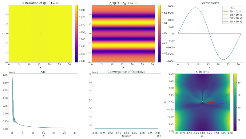
Figure 70. Figure 70: Simulation of (2.1) with under-parametrized H obtained from (2.6) using (EE) with far initialization using GD with line-search. From left to right and top to bottom: f[H](T = 30, x, v), |f[H](T, x, v) − feq(v)|, H and Ef[H](T, x), Ef[H](t, x), Ef[H](t) and, convergence of objective [PITH_FULL_IMAGE:figures/full_fig_p053_70.png] view at source ↗
Figure 71
Figure 71. Figure 71: Simulation of (2.1) with over-parametrized H obtained from (2.6) using (EE) with far initialization using GD with constant stepsize. From left to right and top to bottom: f[H](T = 30, x, v), |f[H](T, x, v) − feq(v)|, H and Ef[H](t, x), Ef[H](t), convergence of objective and, trajectory over the landscape of the objective (yellow dot is initial guess). 53 [PITH_FULL_IMAGE:figures/full_fig_p053_71.png] view at source ↗
Figure 72
Figure 72. Figure 72: Simulation of (2.1) with over-parametrized H obtained from (2.6) using (EE) with near initialization using GD with line-search. From left to right and top to bottom: f[H](T = 30, x, v), |f[H](T, x, v) − feq(v)|, H and Ef[H](t, x), Ef[H](t), convergence of objective and, trajectory over the land￾scape of the objective (yellow dot is initial guess) [PITH_FULL_IMAGE:figures/full_fig_p054_72.png] view at source ↗
Figure 73
Figure 73. Figure 73: Simulation of (2.1) using (EE) with over-parametrized H obtained from (2.6) with near ini￾tialization using GD with constant stepsize. From left to right and top to bottom: f[H](T = 30, x, v), |f[H](T, x, v) − feq(v)|, H and Ef[H](t, x), Ef[H](t), convergence of objective and, trajectory over the land￾scape of the objective (yellow dot is initial guess). 54 [PITH_FULL_IMAGE:figures/full_fig_p054_73.png] view at source ↗
Figure 74
Figure 74. Figure 74: Simulation of (2.1) with over-parametrized H obtained from (2.6) using (EE) with local initialization using GD with line-search. From left to right and top to bottom: f[H](T = 30, x, v), |f[H](T, x, v) − feq(v)|, H and Ef[H](t, x), Ef[H](t), convergence of objective and, trajectory over the land￾scape of the objective (yellow dot is initial guess) [PITH_FULL_IMAGE:figures/full_fig_p055_74.png] view at source ↗
Figure 75
Figure 75. Figure 75: Simulation of (2.1) using (EE) with over-parametrized H obtained from (2.6) with local ini￾tialization using GD with constant stepsize. From left to right and top to bottom: f[H](T = 30, x, v), |f[H](T, x, v) − feq(v)|, H and Ef[H](t, x), Ef[H](t), convergence of objective and, trajectory over the land￾scape of the objective (yellow dot is initial guess). 55 [PITH_FULL_IMAGE:figures/full_fig_p055_75.png] view at source ↗
Figure 76
Figure 76. Figure 76: Simulation of (2.1) with under-parametrized H obtained from (2.6) using (EET) with far initialization using GD with line-search. From left to right and top to bottom: f[H](T = 30, x, v), |f[H](T, x, v) − feq(v)|, H and Ef[H](T, x), Ef[H](t, x), Ef[H](t) and, convergence of objective [PITH_FULL_IMAGE:figures/full_fig_p056_76.png] view at source ↗
Figure 77
Figure 77. Figure 77: Simulation of (2.1) with over-parametrized H obtained from (2.6) using (EET) with far ini￾tialization using GD with constant stepsize. From left to right and top to bottom: f[H](T = 30, x, v), |f[H](T, x, v) − feq(v)|, H and Ef[H](t, x), Ef[H](t), convergence of objective and, trajectory over the land￾scape of the objective (yellow dot is initial guess). 56 [PITH_FULL_IMAGE:figures/full_fig_p056_77.png] view at source ↗
Figure 78
Figure 78. Figure 78: Simulation of (2.1) with over-parametrized H obtained from (2.6) using (EET) with near initialization using GD with line-search. From left to right and top to bottom: f[H](T = 30, x, v), |f[H](T, x, v) − feq(v)|, H and Ef[H](t, x), Ef[H](t), convergence of objective and, trajectory over the land￾scape of the objective (yellow dot is initial guess) [PITH_FULL_IMAGE:figures/full_fig_p057_78.png] view at source ↗
Figure 79
Figure 79. Figure 79: Simulation of (2.1) using (EET) with over-parametrized H obtained from (2.6) with near ini￾tialization using GD with constant stepsize. From left to right and top to bottom: f[H](T = 30, x, v), |f[H](T, x, v) − feq(v)|, H and Ef[H](t, x), Ef[H](t), convergence of objective and, trajectory over the land￾scape of the objective (yellow dot is initial guess). 57 [PITH_FULL_IMAGE:figures/full_fig_p057_79.png] view at source ↗
Figure 80
Figure 80. Figure 80: Simulation of (2.1) with over-parametrized H obtained from (2.6) using (EET) with local initialization using GD with line-search. From left to right and top to bottom: f[H](T = 30, x, v), |f[H](T, x, v) − feq(v)|, H and Ef[H](t, x), Ef[H](t), convergence of objective and, trajectory over the land￾scape of the objective (yellow dot is initial guess) [PITH_FULL_IMAGE:figures/full_fig_p058_80.png] view at source ↗
Figure 81
Figure 81. Figure 81: Simulation of (2.1) using (EET) with over-parametrized H obtained from (2.6) with local ini￾tialization using GD with constant stepsize. From left to right and top to bottom: f[H](T = 30, x, v), |f[H](T, x, v) − feq(v)|, H and Ef[H](t, x), Ef[H](t), convergence of objective and, trajectory over the land￾scape of the objective (yellow dot is initial guess). 58 [PITH_FULL_IMAGE:figures/full_fig_p058_81.png] view at source ↗
read the original abstract

Stabilizing plasma dynamics is a central challenge in magnetic confinement fusion. A common approach is to introduce external electric fields to suppress instabilities in the plasma distribution. However, efficiently identifying such stabilizing fields remains challenging, even for simplified kinetic models such as the Vlasov-Poisson (VP) system. In this work we study plasma stabilization from the perspective of PDE-constrained optimization. Our goal is to understand how the choice of objective function and the underlying kinetic dynamics influence the optimization landscape. First, we analyze the dispersion relation of the VP system and show that it reveals the spectral structure of the dynamics; eliminating unstable modes provides parameter configurations that lie close to the global optimum and serve as effective initial guesses for optimization. Second, we investigate several objective functions for stabilization and compare their optimization landscapes through numerical experiments. Our results show that while different objectives lead to similar stabilizing parameter configurations, objective functions incorporating time-integrated information exhibit more convex-like landscapes and are therefore more favorable for gradient-based optimization methods. These findings provide insight into the design of objective functions for optimization-based plasma control and suggest promising directions for future research on real-time stabilization of kinetic plasma models.

Editorial analysis

A structured set of objections, weighed in public.

Desk editor's note, referee report, simulated authors' rebuttal, and a circularity audit. Tearing a paper down is the easy half of reading it; the pith above is the substance, this is the friction.

Referee Report

2 major / 2 minor

Summary. The manuscript studies PDE-constrained optimization for suppressing instabilities in the Vlasov-Poisson system via external electric fields. It first analyzes the dispersion relation to identify parameter values that eliminate unstable modes and provide effective initial guesses near the global optimum. It then compares several objective functions through numerical experiments on a simplified VP system, reporting that time-integrated objectives (e.g., integrals of norms or energy over [0,T]) produce more convex-like optimization landscapes than instantaneous ones and are therefore preferable for gradient-based methods.

Significance. If the numerical landscape comparison holds under rigorous quantification, the results would offer concrete guidance on objective-function design for optimization-based plasma control, with direct relevance to kinetic models in fusion research. The dispersion-relation analysis for generating high-quality initial guesses is a clear strength, as is the reproducible numerical comparison of multiple objectives on the same VP setup.

major comments (2)
  1. [§4] §4 (Numerical Experiments): The central claim that time-integrated objectives yield more convex-like landscapes rests on qualitative visualization of optimization landscapes and the observation that stabilizing parameters are similar across objectives. No quantitative convexity metrics (Hessian condition numbers, sampled local-minima counts, or gradient-descent success rates from randomized starts) are reported, rendering the inference that these landscapes are 'more favorable for gradient-based optimization methods' interpretive rather than measured.
  2. [§4.1 and §4.2] §4.1 and §4.2: The description of the numerical experiments lacks explicit details on the spatial and velocity discretization of the VP system, the time-stepping scheme, error-control tolerances, and any statistical robustness checks (multiple independent runs or sensitivity to mesh parameters) used to support the convexity comparison. These omissions make it difficult to assess whether the reported landscape differences are robust or discretization artifacts.
minor comments (2)
  1. [§3] The mathematical definitions of the objective functions (instantaneous vs. time-integrated) would benefit from a single, clearly labeled subsection containing their explicit integral expressions and any regularization terms.
  2. [Figures 3-5] Figure captions for the landscape plots should state the precise parameter ranges, number of sampled points, and any smoothing applied, to allow readers to reproduce the visual comparison.
Simulated Author's Rebuttal

2 responses · 0 unresolved

We thank the referee for their constructive and detailed review. We agree that strengthening the quantitative support for the landscape comparison and expanding the numerical details will improve the manuscript. We address each major comment below and indicate planned revisions.

read point-by-point responses
  1. Referee: [§4] §4 (Numerical Experiments): The central claim that time-integrated objectives yield more convex-like landscapes rests on qualitative visualization of optimization landscapes and the observation that stabilizing parameters are similar across objectives. No quantitative convexity metrics (Hessian condition numbers, sampled local-minima counts, or gradient-descent success rates from randomized starts) are reported, rendering the inference that these landscapes are 'more favorable for gradient-based optimization methods' interpretive rather than measured.

    Authors: We acknowledge that the evidence presented for more convex-like landscapes under time-integrated objectives is primarily qualitative, based on visual inspection of the objective surfaces and the consistency of stabilizing parameters across objectives. While these observations support our interpretation, we agree that quantitative metrics would make the claim more rigorous. In the revised manuscript we will add success rates of gradient descent from multiple randomized initial guesses and counts of distinct local minima encountered across repeated optimizations. Full Hessian condition numbers remain computationally expensive for the PDE-constrained setting, but we will include finite-difference estimates of local curvature at sampled points to provide additional quantitative support. revision: yes

  2. Referee: [§4.1 and §4.2] §4.1 and §4.2: The description of the numerical experiments lacks explicit details on the spatial and velocity discretization of the VP system, the time-stepping scheme, error-control tolerances, and any statistical robustness checks (multiple independent runs or sensitivity to mesh parameters) used to support the convexity comparison. These omissions make it difficult to assess whether the reported landscape differences are robust or discretization artifacts.

    Authors: We thank the referee for highlighting these omissions. In the revised version we will expand Sections 4.1 and 4.2 with complete specifications of the spatial and velocity grids (including point counts and domain sizes), the time-stepping scheme and splitting method used for the Vlasov-Poisson system, the error tolerances applied, and results from multiple independent runs with varied random seeds. We will also report a brief mesh-sensitivity study to confirm that the observed differences between objective landscapes persist under refinement and are not discretization artifacts. revision: yes

Circularity Check

0 steps flagged

No significant circularity; claims rest on independent analysis and experiments.

full rationale

The paper derives its conclusions from two independent sources: (1) standard dispersion-relation analysis of the Vlasov-Poisson system that identifies unstable modes and supplies initial guesses near the optimum, and (2) direct numerical optimization experiments that compare landscapes for instantaneous versus time-integrated objective functions. Neither step reduces by construction to a fitted parameter, a self-citation chain, or a renaming of the input; the dispersion relation is an external spectral property, and the landscape comparison is obtained from fresh simulations rather than from quantities defined in terms of the claimed result. The derivation is therefore self-contained against external benchmarks.

Axiom & Free-Parameter Ledger

0 free parameters · 1 axioms · 0 invented entities

The work relies on the standard Vlasov-Poisson model and standard PDE-constrained optimization machinery; no new free parameters, axioms beyond domain assumptions, or invented entities are introduced in the abstract.

axioms (1)
  • domain assumption The Vlasov-Poisson system is an adequate reduced model for studying external-field stabilization of plasma instabilities.
    All analysis and experiments are performed inside this kinetic model.

pith-pipeline@v0.9.0 · 5747 in / 1109 out tokens · 73612 ms · 2026-05-22T19:39:22.556691+00:00 · methodology

discussion (0)

Sign in with ORCID, Apple, or X to comment. Anyone can read and Pith papers without signing in.

Reference graph

Works this paper leans on

57 extracted references · 57 canonical work pages

  1. [1]

    Instantaneous control strategies for magnetically confined fusion plasma

    Giacomo Albi, Giacomo Dimarco, Federica Ferrarese, and Lorenzo Pareschi. “Instantaneous control strategies for magnetically confined fusion plasma”. In: Journal of Computational Physics 527 (2025), p. 113804. issn: 0021-9991. doi: 10.1016/j.jcp.2025.113804 . url: https://www.sciencedirect. com/science/article/pii/S0021999125000877

  2. [2]

    Robust feedback control of collisional plasma dynamics in presence of uncertainties

    Giacomo Albi, Giacomo Dimarco, Federica Ferrarese, and Lorenzo Pareschi. Robust feedback control of collisional plasma dynamics in presence of uncertainties . 2025. arXiv: 2505.19992 [math.NA] . url: https://arxiv.org/abs/2505.19992

  3. [3]

    A tutorial presentation of the two stream instability and Landau damping

    D. Anderson, R. Fedele, and M. Lisak. “A tutorial presentation of the two stream instability and Landau damping”. In: American Journal of Physics (2001). doi: 10.1119/1.1407252

  4. [4]

    Controlling a Vlasov–Poisson Plasma by a Particle-in-Cell Method Based on a Monte Carlo Framework

    Jan Bartsch, Patrik Knopf, Stefania Scheurer, and J¨ org Weber. “Controlling a Vlasov–Poisson Plasma by a Particle-in-Cell Method Based on a Monte Carlo Framework”. In: SIAM Journal on Control and Optimization 62.4 (2024), pp. 1977–2011. doi: 10.1137/23M1563852

  5. [5]

    Semi-Lagrangian schemes for the Vlasov equation on an unstructured mesh of phase space

    N. Besse and E. Sonnendr¨ ucker. “Semi-Lagrangian schemes for the Vlasov equation on an unstructured mesh of phase space”. In: Journal of Computational Physics 191.2 (2003), pp. 341–376. issn: 0021-

  6. [6]

    The weak and strong Lefschetz properties for ArtinianK-algebras

    doi: 10.1016/S0021- 9991(03)00318- 8 . url: https://www.sciencedirect.com/science/ article/pii/S0021999103003188

  7. [7]

    Modeling of active control of external magnetohydrodynamic instabilities

    James Bialek, Allen H. Boozer, M. E. Mauel, and G. A. Navratil. “Modeling of active control of external magnetohydrodynamic instabilities”. In: Physics of Plasmas 8.5 (May 2001), pp. 2170–2180. issn: 1070-664X. doi: 10 . 1063 / 1 . 1362532. url: https : / / pubs . aip . org / aip / pop / article - pdf/8/5/2170/19187304/2170%5C_1%5C_online.pdf

  8. [8]

    Control Methods for the Opti- mization of Plasma Scenarios in a Tokamak

    Jacques Blum, C´ edric Boulbe, Blaise Faugeras, and Holger Heumann. “Control Methods for the Opti- mization of Plasma Scenarios in a Tokamak”. In:IFIP TC7 2015 - 27th Conference on System Modeling and Optimization. Ed. by Lorena Bociu, Jean-Antoine D´ esid´ eri, and Abderrahmane Habbal. Springer International Publishing, 2016, pp. 1–20. isbn: 978-3-319-55...

  9. [9]

    Optimal Design of Equilibrium Solutions of the Vlasov–Poisson System by an External Electric Field

    A. Borz` ı, G. Infante, and G. Mascali. “Optimal Design of Equilibrium Solutions of the Vlasov–Poisson System by an External Electric Field”. In:SIAM Journal on Applied Mathematics 85.1 (2025), pp. 143–

  10. [10]

    doi: 10.1137/24M1643177

  11. [11]

    JAX: composable transformations of Python+NumPy programs

    James Bradbury et al. JAX: composable transformations of Python+NumPy programs . Version 0.6.0

  12. [12]

    url: http://github.com/jax-ml/jax

  13. [13]

    Plasma: The Fourth State of Matter

    KTAL Burm. “Plasma: The Fourth State of Matter”. In: Plasma Chemistry and Plasma Processing 32.2 (2012), pp. 401–407. doi: 10.1007/s11090-012-9356-1

  14. [14]

    Raissi, P

    Xiaofeng Cai, Sebastiano Boscarino, and Jing-Mei Qiu. “High order semi-Lagrangian discontinuous Galerkin method coupled with Runge-Kutta exponential integrators for nonlinear Vlasov dynamics”. In: Journal of Computational Physics 427 (2021), p. 110036. issn: 0021-9991. doi: 10.1016/j.jcp. 2020.110036. url: https://www.sciencedirect.com/science/article/pii...

  15. [15]

    Introduction to plasma physics and controlled fusion

    Francis F Chen. Introduction to plasma physics and controlled fusion . Vol. 1. Springer, 1984. doi: 10.1007/978-1-4757-5595-4

  16. [16]

    High-Frequency Limit of the Inverse Scattering Problem: Asymptotic Convergence from Inverse Helmholtz to Inverse Liouville

    Shi Chen, Zhiyan Ding, Qin Li, and Leonardo Zepeda-N´ u˜ nez. “High-Frequency Limit of the Inverse Scattering Problem: Asymptotic Convergence from Inverse Helmholtz to Inverse Liouville”. In: SIAM Journal on Imaging Sciences 16.1 (2023), pp. 111–143. doi: 10.1137/22M147075X

  17. [17]

    The integration of the Vlasov equation in configuration space

    Chio-Zong Cheng and Georg Knorr. “The integration of the Vlasov equation in configuration space”. In: Journal of Computational Physics 22.3 (1976), pp. 330–351. issn: 0021-9991. doi: 10 . 1016 / 0021 - 9991(76 ) 90053 - X. url: https : / / www . sciencedirect . com / science / article / pii / 002199917690053X

  18. [18]

    Discontinuous Galerkin semi-Lagrangian method for Vlasov-Poisson

    N. Crouseilles, M. Mehrenberger, and Vecil, F. “Discontinuous Galerkin semi-Lagrangian method for Vlasov-Poisson”. In: ESAIM: Proc. 32 (2011), pp. 211–230. doi: 10.1051/proc/2011022. 19

  19. [19]

    Magnetic control of tokamak plasmas through deep reinforcement learning

    Jonas Degrave et al. “Magnetic control of tokamak plasmas through deep reinforcement learning”. In: Nature 602.7897 (2022), pp. 414–419. doi: 10.1038/s41586-021-04301-9

  20. [20]

    A performance comparison of semi-Lagrangian discontinuous Galerkin and spline based Vlasov solvers in four dimensions

    Lukas Einkemmer. “A performance comparison of semi-Lagrangian discontinuous Galerkin and spline based Vlasov solvers in four dimensions”. In: Journal of Computational Physics 376 (2019), pp. 937–

  21. [21]

    doi: 10.1016/j.jcp.2018.10.012

    issn: 0021-9991. doi: 10.1016/j.jcp.2018.10.012 . url: https://www.sciencedirect.com/ science/article/pii/S0021999118306697

  22. [22]

    Control of instability in a Vlasov- Poisson system through an external electric field

    Lukas Einkemmer, Qin Li, Cl´ ement Mouhot, and Yukun Yue. “Control of instability in a Vlasov- Poisson system through an external electric field”. In: Journal of Computational Physics 530 (2025), p. 113904. issn: 0021-9991. doi: 10.1016/j.jcp.2025.113904 . url: https://www.sciencedirect. com/science/article/pii/S0021999125001871

  23. [23]

    Suppressing instability in a Vlasov–Poisson system by an external electric field through constrained optimization

    Lukas Einkemmer, Qin Li, Li Wang, and Yang Yunan. “Suppressing instability in a Vlasov–Poisson system by an external electric field through constrained optimization”. In: Journal of Computational Physics 498 (2024), p. 112662. issn: 0021-9991. doi: 10.1016/j.jcp.2023.112662 . url: https: //www.sciencedirect.com/science/article/pii/S002199912300757X

  24. [24]

    Optimal Transport Based Seismic Inversion:Beyond Cycle Skip- ping

    Bj¨ orn Engquist and Yunan Yang. “Optimal Transport Based Seismic Inversion:Beyond Cycle Skip- ping”. In: Communications on Pure and Applied Mathematics 75.10 (2022), pp. 2201–2244. doi: 10.1002/cpa.21990. url: https://onlinelibrary.wiley.com/doi/abs/10.1002/cpa.21990

  25. [25]

    Comparison of Eulerian Vlasov solvers

    Francis Filbet and Eric Sonnendr¨ ucker. “Comparison of Eulerian Vlasov solvers”. In:Computer Physics Communications 150.3 (2003), pp. 247–266. issn: 0010-4655. doi: 10.1016/S0010-4655(02)00694-X. url: https://www.sciencedirect.com/science/article/pii/S001046550200694X

  26. [26]

    Numerical methods for the Vlasov equation

    Francis Filbet and Eric Sonnendr¨ ucker. “Numerical methods for the Vlasov equation”. In: Numerical Mathematics and Advanced Applications: Proceedings of ENUMATH 2001 the 4th European Conference on Numerical Mathematics and Advanced Applications Ischia, July 2001. Springer Milan, 2003, pp. 459–

  27. [27]

    doi: 10.1007/978-88-470-2089-4_43

    isbn: 978-88-470-2089-4. doi: 10.1007/978-88-470-2089-4_43

  28. [28]

    Plasma physics: an introduction

    Richard Fitzpatrick. Plasma physics: an introduction. 2nd edition. CRC Press, Taylor & Francis Group,

  29. [29]

    doi: 10.1201/9781003268253

    isbn: 978-1-4665-9426-5. doi: 10.1201/9781003268253

  30. [30]

    Plasma: the fourth state of matter

    D Frank-Kamenetskii. Plasma: the fourth state of matter . Springer Science & Business Media, 2012. doi: 10.1007/978-1-4684-1896-5

  31. [31]

    Freidberg

    Jeffrey P. Freidberg. Plasma Physics and Fusion Energy . Cambridge University Press, 2007. isbn: 9780511755705. doi: 10.1017/CBO9780511755705

  32. [32]

    On the controllability of the Vlasov–Poisson system

    Olivier Glass. “On the controllability of the Vlasov–Poisson system”. In: Journal of Differential Equa- tions 195.2 (2003), pp. 332–379. issn: 0022-0396. doi: 10 . 1016 / S0022 - 0396(03 ) 00066 - 4. url: https://www.sciencedirect.com/science/article/pii/S0022039603000664

  33. [33]

    On the controllability of the Vlasov–Poisson system in the presence of external force fields

    Olivier Glass and Daniel Han-Kwan. “On the controllability of the Vlasov–Poisson system in the presence of external force fields”. In: Journal of Differential Equations 252.10 (2012), pp. 5453–5491. issn: 0022-0396. doi: 10 . 1016 / j . jde . 2012 . 02 . 007. url: https : / / www . sciencedirect . com / science/article/pii/S0022039612000848

  34. [34]

    Asymptotic Stability of Equilibria for Screened Vlasov–Poisson Systems via Pointwise Dispersive Estimates

    Daniel Han-Kwan, Toan T. Nguyen, and Fr´ ed´ eric Rousset. “Asymptotic Stability of Equilibria for Screened Vlasov–Poisson Systems via Pointwise Dispersive Estimates”. In: Annals of PDE 7.2 (2021), Paper No. 18, 37 pp. doi: 10.1007/s40818-021-00110-5

  35. [35]

    Nonlinear stability of fluid and plasma equilibria

    Darryl D. Holm, Jerrold E. Marsden, Tudor Ratiu, and Alan Weinstein. “Nonlinear stability of fluid and plasma equilibria”. In: Physics Reports 123.1 (1985), pp. 1–116. issn: 0370-1573. doi: 10.1016/ 0370 - 1573(85 ) 90028 - 6. url: https : / / www . sciencedirect . com / science / article / pii / 0370157385900286

  36. [36]

    Nuclear fusion in dense plasmas

    Setsuo Ichimaru. “Nuclear fusion in dense plasmas”. In: Reviews of Modern Physics 65.2 (1993), pp. 255–299. doi: 10 . 1103 / RevModPhys . 65 . 255. url: https : / / link . aps . org / doi / 10 . 1103 / RevModPhys.65.255

  37. [37]

    Dynamic stabilization of plasma instability

    S. Kawata, T. Karino, and Y.J. Gu. “Dynamic stabilization of plasma instability”. In: High Power Laser Science and Engineering 7 (2019), e3. doi: 10.1017/hpl.2018.61. 20

  38. [38]

    A Splitting Algorithm for Vlasov Simulation with Filamentation Filtration

    A.J. Klimas and W.M. Farrell. “A Splitting Algorithm for Vlasov Simulation with Filamentation Filtration”. In: Journal of Computational Physics 110.1 (1994), pp. 150–163. issn: 0021-9991. doi: 10 . 1006 / jcph . 1994 . 1011. url: https : / / www . sciencedirect . com / science / article / pii / S0021999184710114

  39. [39]

    Absence of recurrence in Fourier–Fourier transformed Vlasov–Poisson simulations

    Alexander J. Klimas and Adolfo. F. Vi˜ nas. “Absence of recurrence in Fourier–Fourier transformed Vlasov–Poisson simulations”. In: Journal of Plasma Physics 84.4 (2018), p. 905840405. doi: 10.1017/ S0022377818000776

  40. [40]

    Confined steady states of a Vlasov-Poisson plasma in an infinitely long cylinder

    Patrik Knopf. “Confined steady states of a Vlasov-Poisson plasma in an infinitely long cylinder”. In: Mathematical Methods in the Applied Sciences 42.18 (2019), pp. 6369–6384. doi: 10.1002/mma.5728. url: https://onlinelibrary.wiley.com/doi/abs/10.1002/mma.5728

  41. [41]

    Optimal control of a Vlasov–Poisson plasma by an external magnetic field

    Patrik Knopf. “Optimal control of a Vlasov–Poisson plasma by an external magnetic field”. In: Calculus of Variations and Partial Differential Equations 57.5 (2018). doi: 10.1007/s00526-018-1407-x

  42. [42]

    Signori, Optimal distributed control of an extended model o f tumor growth with logarithmic potential, Appl

    Patrik Knopf and J¨ org Weber. “Optimal Control of a Vlasov–Poisson Plasma by Fixed Magnetic Field Coils”. In: Applied Mathematics & Optimization 81.3 (2020), pp. 961–988. doi: 10.1007/s00245- 018-9526-5

  43. [43]

    Plasma Physics for Nuclear Fusion

    Kenro Miyamoto. Plasma Physics for Nuclear Fusion . Revised Ed. The MIT Press, 1989. isbn: 978-0- 26-263117-4

  44. [44]

    Magnetic measurements on the TCV Tokamak

    J.-M. Moret et al. “Magnetic measurements on the TCV Tokamak”. In: Review of Scientific Instruments 69.6 (June 1998), pp. 2333–2348. issn: 0034-6748. doi: 10.1063/1.1148940 . url: https://pubs. aip.org/aip/rsi/article-pdf/69/6/2333/19105874/2333%5C_1%5C_online.pdf

  45. [45]

    On Landau damping

    Cl´ ement Mouhot and C´ edric Villani. “On Landau damping”. In: Acta Mathematica 207.1 (2011), pp. 29–201. doi: 10.1007/s11511-011-0068-9

  46. [46]

    Introduction to plasma theory

    Dwight Roy Nicholson. Introduction to plasma theory . Vol. 1. Wiley New York, 1983

  47. [47]

    Jorge Nocedal and Stephen J. Wright. Numerical Optimization. Springer Series in Operations Research and Financial Engineering. 2nd Ed. New York, NY: Springer, 2006. isbn: 978-0-387-30303-1. doi: 10.1007/978-0-387-40065-5

  48. [48]

    Nonlinear interaction of a small cold beam and a plasma

    T.M. O’Neil, J.H. Winfrey, and J.H. Malmberg. “Nonlinear interaction of a small cold beam and a plasma”. In: The Physics of Fluids 14.6 (1971), pp. 1204–1212. doi: 10.1063/1.1693587

  49. [49]

    Electrostatic instabilities of a uniform non-Maxwellian plasma

    Oliver Penrose. “Electrostatic instabilities of a uniform non-Maxwellian plasma”. In: The Physics of Fluids 3.2 (1960), pp. 258–265. doi: 10.1063/1.1706024

  50. [50]

    Positivity preserving semi-Lagrangian discontinuous Galerkin for- mulation: theoretical analysis and application to the Vlasov–Poisson system

    Jing-Mei Qiu and Chi-Wang Shu. “Positivity preserving semi-Lagrangian discontinuous Galerkin for- mulation: theoretical analysis and application to the Vlasov–Poisson system”. In: Journal of Compu- tational Physics 230.23 (2011), pp. 8386–8409. doi: 10.1016/j.jcp.2011.07.018

  51. [51]

    A positivity-preserving high-order semi-Lagrangian dis- continuous Galerkin scheme for the Vlasov–Poisson equations

    James A. Rossmanith and David C. Seal. “A positivity-preserving high-order semi-Lagrangian dis- continuous Galerkin scheme for the Vlasov–Poisson equations”. In: Journal of Computational Physics 230.16 (2011), pp. 6203–6232. issn: 0021-9991. doi: 10 . 1016 / j . jcp . 2011 . 04 . 018. url: https : //www.sciencedirect.com/science/article/pii/S0021999111002579

  52. [52]

    Avoiding fusion plasma tearing instability with deep reinforcement learning

    Jaemin Seo et al. “Avoiding fusion plasma tearing instability with deep reinforcement learning”. In: Nature 626.8000 (2024), pp. 746–751. doi: 10.1038/s41586-024-07024-9

  53. [53]

    Multimodal Prediction of Tearing Instabilities in a Tokamak

    Jaemin Seo et al. “Multimodal Prediction of Tearing Instabilities in a Tokamak”. In: 2023 International Joint Conference on Neural Networks (IJCNN). 2023, pp. 1–8. isbn: 978-1-6654-8867-9. doi: 10.1109/ IJCNN54540.2023.10191359

  54. [54]

    The semi-Lagrangian method for the numerical resolution of the Vlasov equation

    Eric Sonnendr¨ ucker, Jean Roche, Pierre Bertrand, and Alain Ghizzo. “The semi-Lagrangian method for the numerical resolution of the Vlasov equation”. In: Journal of Computational Physics 149.2 (1999), pp. 201–220. doi: 10.1006/jcph.1998.6148 . url: https://www.sciencedirect.com/science/ article/pii/S0021999198961484

  55. [55]

    Magnetic control of magnetohydrodynamic instabilities in tokamaks

    E. J. Strait. “Magnetic control of magnetohydrodynamic instabilities in tokamaks”. In: Physics of Plasmas 22.2 (Nov. 2014), p. 021803. issn: 1070-664X. doi: 10 . 1063 / 1 . 4902126. url: https : //pubs.aip.org/aip/pop/article- pdf/doi/10.1063/1.4902126/16137245/021803%5C_1%5C_ online.pdf. 21

  56. [56]

    Velocity inversion by differential semblance optimization

    W. W. Symes and J. J. Carazzone. “Velocity inversion by differential semblance optimization”. In: GEOPHYSICS 56.5 (1991), pp. 654–663. doi: 10.1190/1.1443082 . url: https://library.seg. org/doi/10.1190/1.1443082

  57. [57]

    Particle simulation of plasmas: review and advances

    J P Verboncoeur. “Particle simulation of plasmas: review and advances”. In: Plasma Physics and Controlled Fusion 47.5A (2005), A231. doi: 10.1088/0741-3335/47/5A/017. A Comparison between L2 and KL Another possible function is to use the L2 disparity: J (f[H]) = 1 2 ∥fT [H] − feq∥2 L2(x,v) = 1 2 Z Lv −Lv (f[H](T, x, v) − feq(v))2dxdv (L2) J (f[H]) = 1 2 Z...