REVIEW 4 major objections 6 minor 29 references
A Unified Alternating Optimization Framework for Joint Sensor and Actuator Configuration in LQG Systems
T0 review · 4 major / 6 minor · reviewed 2026-08-16 · deepseek-v4-flash
Pith's one-line read LQG sensor and actuator design becomes a differentiable optimization problem
desk verdict Useful continuous co-design formulation and solid gradient derivations, but the Algorithm 2 convergence proof rests on an invalid spectral abscissa claim. read the letter →
The pith
A machine-rendered reading of the paper's core claim, the machinery that carries it, and where it could break.
The reading
What carries the argument
The central object is the pair of continuous-time algebraic Riccati equations (CAREs) for the optimal observer and controller, whose unique positive-definite solutions $X$ and $P$ exist under the stabilizability and detectability assumption. The paper perturbs $B$ and $C$ through these CAREs, rearranges trace identities, and obtains gradient formulas expressed through Lyapunov equations; this is what turns the implicit LQG cost into an explicitly differentiable objective. The optimization machinery is an ADMM splitting that separates the smooth nonconvex LQG term from the convex nonsmooth configuration cost, with auxiliary-variable updates that have closed forms for the three scenarios considered.
What would settle it
A numerical scan that approaches the boundary of the stabilizable region and finds bounded LQG cost while the optimal feedback gain grows without bound would falsify the coercivity premise behind Theorem 4.
Extended reading notes
Core claim
The central claim is that the LQG cost $J_{\mathrm{LQG}}$, despite depending on $B$ and $C$ only implicitly through two continuous-time algebraic Riccati equations, has closed-form gradients: $\partial J_{\mathrm{LQG}}/\partial B = -2P(G_1+G_2)PBR^{-1}$ and $\partial J_{\mathrm{LQG}}/\partial C = -2\Pi_v^{-1}CX(H_1+H_2)X$, where $P,X$ are the Riccati solutions and $G_1,G_2,H_1,H_2$ solve Lyapunov equations built from the optimal closed-loop and observer matrices. Theorem 3 converts these gradients into necessary first-order optimality conditions for the constrained joint configuration problem, and Theorem 4 states that the accumulation point of Algorithm 2, an ADMM-based alternating optimization, satisfies these conditions and is therefore at least a stationary point. The paper also gives closed-form proximal updates for three representative scenarios: soft thresholding for $\ell^1$ sparsity, singular value thresholding for the nuclear norm, and a mask projection for structure constraints.
Load-bearing premise
The proof that Algorithm 2 reaches a stationary point rests on two unsupported premises: that the LQG cost diverges at the boundary of the stabilizable/detectable region even when the optimal gains diverge, and that each alternating update never increases the total cost.
Editorial extensions
If this is right
- Designers can optimize sensor and actuator matrices from scratch, with no predefined candidate set, while the stabilizability and detectability constraints are enforced by the optimization itself.
- A returned configuration $(B^*,C^*)$ can be checked for stationarity by directly evaluating the two gradient formulas and the corresponding normal-cone conditions.
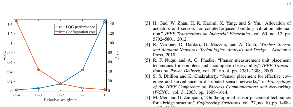
- Varying the relative weight $\gamma$ traces a performance-versus-configuration-cost frontier, as demonstrated numerically for sparsity, low-rank, and structure-constrained designs.
- Low-rank solutions come with explicit factorizations $B=B_1B_2$ and $C=C_1C_2$, so the designed matrices translate directly into a reduced set of actuators and sensors.
- Because the outer loop alternates and each inner ADMM update is either a smooth gradient step or a convex proximal step, the framework can be embedded in numerical solvers with modest per-iteration cost.
Reading between the lines
- The same Riccati-perturbation derivation is likely to produce analogous gradient formulas for discrete-time LQG or $H_2$ performance, although the paper does not state these extensions.
- The stationarity guarantee is local, so global optimality should not be assumed; restarting Algorithm 2 from several initial pairs is a natural safeguard that the paper does not discuss.
- If the true design problem is binary (a sensor or actuator is either installed or not), the continuous matrices returned by this framework would need a rounding or mixed-integer layer, which the paper leaves implicit.
- The coercivity premise behind the boundary argument is directly testable: a numerical scan of near-unstabilizable pairs would reveal whether the LQG cost actually diverges when the optimal feedback gain itself blows up.
Signed reviews
Editorial analysis
A structured set of objections, weighed in public.
Referee Report
Summary. The paper studies the joint design of the actuator matrix B and sensor matrix C for a continuous-time LQG system without assuming a pre-specified set of candidate components. The objective is J(B,C)=J_LQG+γ(Φ(B)+Ψ(C)) subject to convex configuration constraints and to stabilizability/detectability of (A,B) and (A,C). The main theoretical results are analytic gradient formulas for J_LQG with respect to B and C (Theorems 1 and 2), KKT-type necessary conditions (Theorem 3), and an ADMM-based alternating optimization algorithm (Algorithm 2) that is claimed to converge to a stationary point of the problem (Theorem 4). The paper also specializes the proximal updates to three scenarios: ℓ1 sparsity promotion, nuclear-norm low-rank promotion, and support-structure constraints. Numerical experiments on the REA1 benchmark compute returned matrices and verify the corresponding stationarity residuals.
Significance. The analytic gradient formulas are the paper's clearest contribution: they are derived directly from the CARE/Lyapunov equations, contain no fitted parameters, and provide a practical stationarity check. The KKT conditions and the closed-form ADMM updates for the three scenarios are useful building blocks. The numerical verification is also a strength: the authors check the KKT residuals of the returned solutions rather than only plotting objective decrease. However, the central convergence claim of Algorithm 2 (Theorem 4) is not proven as written: its proof depends on an invalid step in Proposition 1 and on an unproven monotonicity assertion. The gradient and stationarity results of Theorems 1–3 appear sound, but the algorithmic guarantee needs substantial repair before the paper can be accepted.
major comments (4)
- [III.A, Proposition 1, Eq. (28)] The proof of Proposition 1 is invalid. Equation (28) asserts σ(A+B_iK_i^*)→σ(A+BK^*)=0 as B_i→B∈∂S, but K_i^*=−R^{-1}B_i^TP_i depends on the CARE solution P_i, and P_i may diverge as stabilizability is lost. For example, with scalar A=1, B_i=ε_i→0, and Q=R=1, the CARE solution is P_i=(1+√(1+ε_i^2))/ε_i^2, so A+B_iK_i^*=1−ε_i^2P_i=−√(1+ε_i^2)→−1, not 0. Consequently the Lyapunov lower bound (30) does not force tr(P_i)→∞. Because Proposition 1 is the basis for the coercivity used to keep iterates in S and to ensure accumulation points in Theorem 4, Theorem 4 is not established by the argument given.
- [III.A, Remark 4, Eq. (36)] Remark 4 asserts the monotone decrease J(B_{h+1},C_h)≤J(B_h,C_h), but this does not follow from the ADMM inner loop as implemented. Algorithm 2 stops the inner ADMM at fixed positive tolerances ǫpri and ǫdual, so B_{h+1}=M_k is not an exact minimizer of (32); for a nonconvex smooth term, the ADMM stationarity relations (38)–(39) do not imply a decrease of the original objective J. The cited reference [24] concerns convergence of ADMM to a stationary point of the augmented or original problem under additional conditions; it does not supply the outer monotonicity (36). Without (36), the outer iterates need not converge, so the existence of the accumulation point (B^*,C^*) assumed in Theorem 4 is unjustified.
- [III.A, Theorem 4 proof, Eqs. (38)–(44)] The proof of Theorem 4 has a double-limit gap. It derives stationarity for the inner iterate B_{k+1} while the outer variable is fixed at C_h, but then writes C^* and passes k→∞ and h→∞ simultaneously without justifying the interchange. It also replaces ∂J(B_{k+1},C^*)/∂B by ∂J(M_{k+1},C^*)/∂B on the strength of ‖B_{k+1}−M_{k+1}‖≤ǫpri; this requires a Lipschitz estimate for the gradient and a limit argument as ǫpri→0, and similarly for ρ(M_{k+1}−M_k)→0 as ǫdual→0. The tolerances are fixed positive constants in Algorithm 2, so the claimed limit is not immediate. As written, the conclusion that (B^*,C^*) satisfies (44)–(45) does not follow.
- [III.A, Theorem 3] The second, more specific part of Theorem 3 represents the normal cone N_{Ω_B}(B) as the set of all linear combinations of gradients of the equality and inequality descriptions with μ^j_B≥0. This representation requires a constraint qualification (for example, a Slater-type condition for the convex description); the statement and proof do not mention any such qualification. Without it, the displayed KKT conditions can fail at nonregular feasible points. The three concrete scenarios studied later have simple constraint sets where the issue is benign, but the general theorem as stated is missing an assumption.
minor comments (6)
- [II.A / Theorem 2] In Theorem 2, 'Given a constant actuator matrix B∈D, for any sensor matrix C∈S' should be 'B∈S and C∈D'; the symbols appear swapped.
- [III.A, Theorem 1 proof] In the increment of the CARE in the proof of Theorem 1, the term '∆P A^T' should read '∆P A'.
- [III.D, Lemma 5 proof] The proof of Lemma 5 begins 'Given that Φ(B)=0', but in this scenario Φ(M)=‖M‖_F^2; the zero-cost claim is a typo.
- [IV.C] The displayed matrices B^* and C^* for the structure-constrained scenario appear to have misaligned rows and columns: B^* is printed with a single 0 in the first row, and C^* appears to have five rows. Please correct the typesetting.
- [III.A, Algorithm 1] Algorithm 1 does not specify a stopping criterion for the inner gradient descent, although Theorem 4's proof treats B_{k+1} as an exact stationary point of (37); the dependence on the inner tolerance should be stated.
- [III.A, Remark 4] The choice of ρ is only described as 'sufficiently large'; the simulations fix ρ=1 with no sensitivity study, so the practical reliability of the convexification argument is not demonstrated.
Circularity Check
No significant circularity: the gradient and KKT derivations are self-contained, and the stationarity verification is a post-hoc consistency check, not an input-equivalent prediction.
full rationale
The paper's central results — the LQG gradient formulas in Theorems 1 and 2 — are derived by increment analysis of the dual algebraic Riccati equations (5)–(6) and by solving auxiliary Lyapunov equations. No fitted constants appear in this derivation, no target value is assumed, and no load-bearing self-citation is used. Theorem 3 obtains KKT conditions by applying standard variational-inequality theory [20] to these gradients, which is a direct mathematical consequence rather than a renaming of a known result. Theorem 4's proof takes the ADMM iterates and checks that, in the limit of vanishing residuals, they satisfy the same first-order conditions; the simulation sections verify the returned matrices against Corollaries 1–3. This is a consistency check of the numerical output, not a 'prediction' forced by construction. The concerns noted by the skeptical reader — Proposition 1's coercivity proof relying on the questionable limit sigma(A + B_i K_i^*) -> 0 in Eq. (28), and the asserted but unproven monotone decrease in Remark 4 — are correctness or rigor gaps in the convergence argument, not circular reductions: they do not make the gradient formulas, KKT conditions, or stationarity checks equivalent to their inputs by definition. Since no step identified reduces to its own inputs and no self-citation chain carries the derivation, the circularity score is 0.
Assumptions & free parameters
free parameters (2)
- Relative cost weight gamma =
0.01 in the main runs; varied in tradeoff curves
- ADMM penalty parameter rho =
1 in all simulations
assumptions (5)
- domain assumption Assumption 1: (A,B) stabilizable and (A,C) detectable for the configured matrices.
- domain assumption Noise covariance Pi_w and weight Q are strictly positive definite.
- standard math The LQG optimal controller and observer are given by the two decoupled CAREs (5) and (6), i.e., the separation principle.
- domain assumption Configuration costs Phi and Psi and constraint sets Omega_B and Omega_C are convex.
- ad hoc to paper Constraint qualification holds for the explicit equality and inequality description of Omega_B and Omega_C in Theorem 3.
Cite this review
Pith. "Pith review of A Unified Alternating Optimization Framework for Joint Sensor and Actuator Configuration in LQG Systems." pith.science (2026). https://pith.science/paper/7KK3EYFY
@misc{pith2026250418731,
  author       = {Pith},
  title        = {Pith review of: A Unified Alternating Optimization Framework for Joint Sensor and Actuator Configuration in LQG Systems},
  year         = {2026},
  howpublished = {\url{https://pith.science/paper/7KK3EYFY}},
  note         = {Machine review of arXiv:2504.18731}
}
read the original abstract
This paper fills a gap in the literature by considering a joint sensor and actuator configuration problem under the linear quadratic Gaussian (LQG) performance without assuming a predefined set of candidate components. Different from the existing research, which primarily focuses on selecting or placing sensors and actuators from a fixed group, we consider a more flexible formulation where these components must be designed from scratch, subject to general-form configuration costs and constraints. To address this challenge, we first analytically characterize the gradients of the LQG performance with respect to the sensor and actuator matrices using algebraic Riccati equations. Subsequently, we derive first-order optimality conditions based on the Karush-Kuhn-Tucker (KKT) analysis and develop a unified alternating direction method of multipliers (ADMM)-based alternating optimization framework to address the general-form sensor and actuator configuration problem. Furthermore, we investigate three representative scenarios: sparsity promoting configuration, low-rank promoting configuration, and structure-constrained configuration. For each scenario, we provide in-depth analysis and develop tailored computational schemes. The proposed framework ensures numerical efficiency and adaptability to various design constraints and configuration costs, making it well-suited for integration into numerical solvers.
Figures


Figures from the paper (3 more)


Reference graph
Works this paper leans on
-
[24]
Global convergence of ADMM in nonconvex nonsmooth optimization,
Y . Wang, W. Yin, and J. Zeng, “Global convergence of ADMM in nonconvex nonsmooth optimization,” Journal of Scientific Computing , vol. 78, pp. 29–63, 2019
work page 2019
-
[1]
An in te- grated framework for autonomous sensor placement with aeri al robots,
B. Stephens, H.-N. Nguyen, S. Hamaza, and M. Kovac, “An in te- grated framework for autonomous sensor placement with aeri al robots,” IEEE/ASME Transactions on Mechatronics , vol. 28, no. 1, pp. 38–49, 2022
work page 2022
-
[2]
T. Meng, J. Huang, C.-M. Chew, D. Y ang, and Z. Zhong, “Confi guration and design schemes of environmental sensing and vehicle com puting systems for automated driving: A review,” IEEE Sensors Journal , vol. 23, no. 14, pp. 15 305–15 320, 2023
work page 2023
-
[3]
Allocat ion of actuators and sensors for coupled-adjacent-building vibr ation attenua- tion,
H. Gao, W. Zhan, H. R. Karimi, X. Y ang, and S. Yin, “Allocat ion of actuators and sensors for coupled-adjacent-building vibr ation attenua- tion,” IEEE Transactions on Industrial Electronics , vol. 60, no. 12, pp. 5792–5801, 2012
work page 2012
-
[4]
R. V erdone, D. Dardari, G. Mazzini, and A. Conti, Wireless Sensor and Actuator Networks: Technologies, Analysis and Design . Academic Press, 2010
work page 2010
-
[5]
Phasor measurement unit pla cement techniques for complete and incomplete observability,
R. F. Nuqui and A. G. Phadke, “Phasor measurement unit pla cement techniques for complete and incomplete observability,” IEEE Transac- tions on Power Delivery , vol. 20, no. 4, pp. 2381–2388, 2005
work page 2005
-
[6]
Sensor placement for e ffective cov- erage and surveillance in distributed sensor networks,
S. S. Dhillon and K. Chakrabarty, “Sensor placement for e ffective cov- erage and surveillance in distributed sensor networks,” in Proceedings of the IEEE Conference on Wireless Communications and Netwo rking (WCNC), vol. 3, 2003, pp. 1609–1614
work page 2003
-
[7]
On the optimal sensor placement te chniques for a bridge structure,
M. Meo and G. Zumpano, “On the optimal sensor placement te chniques for a bridge structure,” Engineering Structures, vol. 27, no. 10, pp. 1488– 1497, 2005
work page 2005
Show all 29 references
-
[8]
Sensor selection s trategies for state estimation in energy constrained wireless sensor networks,
Y . Mo, R. Ambrosino, and B. Sinopoli, “Sensor selection s trategies for state estimation in energy constrained wireless sensor networks,” Automatica, vol. 47, no. 7, pp. 1330–1338, 2011
2011
-
[9]
Stochast ic sensor scheduling for energy constrained estimation in multi-hop wireless sensor networks,
Y . Mo, E. Garone, A. Casavola, and B. Sinopoli, “Stochast ic sensor scheduling for energy constrained estimation in multi-hop wireless sensor networks,” IEEE Transactions on Automatic Control , vol. 56, no. 10, pp. 2489–2495, 2011
2011
-
[10]
Sensor plac ement for optimal kalman filtering: Fundamental limits, submodulari ty, and algo- rithms,
V . Tzoumas, A. Jadbabaie, and G. J. Pappas, “Sensor plac ement for optimal kalman filtering: Fundamental limits, submodulari ty, and algo- rithms,” in Proceedings of the American Control Conference (ACC) , 2016, pp. 191–196
2016
-
[11]
Minimal actuator placement with bounds on control effort,
V . Tzoumas, M. A. Rahimian, G. J. Pappas, and A. Jadbabai e, “Minimal actuator placement with bounds on control effort,” IEEE Transactions on Control of Network Systems , vol. 3, no. 1, pp. 67–78, 2015
2015
-
[12]
Actuator placement in networks using opti mal control performance metrics,
T. Summers, “Actuator placement in networks using opti mal control performance metrics,” in Proceedings of the 55th IEEE Conference on Decision and Control (CDC) , 2016, pp. 2703–2708
2016
-
[13]
Sensor and actuato r placement for linear systems based on H2 and H∞ optimization,
U. M¨ unz, M. Pfister, and P . Wolfrum, “Sensor and actuato r placement for linear systems based on H2 and H∞ optimization,” IEEE Transactions on Automatic Control , vol. 59, no. 11, pp. 2984–2989, 2014
2014
-
[14]
Al locating sensors and actuators via optimal estimation and control,
J. A. Taylor, N. Luangsomboon, and D. Fooladivanda, “Al locating sensors and actuators via optimal estimation and control,” IEEE Trans- actions on Control Systems Technology , vol. 25, no. 3, pp. 1060–1067, 2016
2016
-
[15]
LQG con- trol and sensing co-design,
V . Tzoumas, L. Carlone, G. J. Pappas, and A. Jadbabaie, “ LQG con- trol and sensing co-design,” IEEE Transactions on Automatic Control , vol. 66, no. 4, pp. 1468–1483, 2020
2020
-
[16]
Joint sensor and actua tor placement for infinite-horizon LQG control,
L. Huang, J. Wu, Y . Mo, and L. Shi, “Joint sensor and actua tor placement for infinite-horizon LQG control,” IEEE Transactions on Automatic Control, vol. 67, no. 1, pp. 398–405, 2021
2021
-
[17]
Optimal senso r and actuator selection using balanced model reduction,
K. Manohar, J. N. Kutz, and S. L. Brunton, “Optimal senso r and actuator selection using balanced model reduction,” IEEE Transactions on Automatic Control , vol. 67, no. 4, pp. 2108–2115, 2021
2021
-
[18]
B. D. Anderson and J. B. Moore, Optimal Control: Linear Quadratic Methods. Courier Corporation, 2007
2007
-
[19]
LQG stable stabil izing control: Some recent results,
R. Arelhi, M. Johnson, and J. Wilkie, “LQG stable stabil izing control: Some recent results,” in Proceedings of the 36th IEEE Conference on Decision and Control (CDC) , vol. 2, 1997, pp. 1431–1436
1997
-
[20]
Boyd and L
S. Boyd and L. V andenberghe, Convex Optimization . Cambridge University Press, 2004
2004
-
[21]
Upper and lower bounds on the sol ution of the algebraic Riccati equation,
K. Y asuda and K. Hirai, “Upper and lower bounds on the sol ution of the algebraic Riccati equation,” IEEE Transactions on Automatic Control , vol. 24, no. 3, pp. 483–487, 1979
1979
-
[22]
Nocedal and S
J. Nocedal and S. J. Wright, Numerical Optimization. New Y ork, NY: Springer, 1999
1999
-
[23]
J. F. Bard, Practical Bilevel Optimization: Algorithms and Applicati ons. Springer Science & Business Media, 2013
2013
-
[25]
Optimally sparse representat ion in general (nonorthogonal) dictionaries via ℓ1 minimization,
D. L. Donoho and M. Elad, “Optimally sparse representat ion in general (nonorthogonal) dictionaries via ℓ1 minimization,” Proceedings of the National Academy of Sciences , vol. 100, no. 5, pp. 2197–2202, 2003
2003
-
[26]
R. T. Rockafellar, Convex Analysis. Princeton University Press, 1997
1997
-
[27]
D. C. Lay, Linear Algebra and Its Applications . Pearson Education India, 2003
2003
-
[28]
Characterization of the subdifferentia l of some matrix norms,
G. A. Watson, “Characterization of the subdifferentia l of some matrix norms,” Linear Algebra Appl , vol. 170, no. 1, pp. 33–45, 1992
1992
-
[29]
Description of the bench mark examples in COMPleib 1.0 (Tech. Report),
F. Leibfritz and W. Lipinski, “Description of the bench mark examples in COMPleib 1.0 (Tech. Report),” Trier: University of Trier , 2003
2003
Reviewed August 16, 2026 · model on record in the stance chip above.
Discussion (0). Continue with ORCID to comment.