REVIEW 3 major objections 5 minor 46 references
An Unsupervised Learning Method for Radio Interferometry Deconvolution
T0 review · 3 major / 5 minor · reviewed 2026-08-15 · deepseek-v4-flash
Pith's one-line read The central claim is that a convolutional network can serve as the sparsifying dictionary inside the split Bregman solver, making unsupervised radio-interferometric deconvolution of faint extended sources possible without labeled training…
desk verdict Genuinely new unsupervised deep-dictionary deconvolution architecture, but the headline DR gains rest on residual metrics, not ground-truth error, and the CS justification is asserted rather than verified. read the letter →
The pith
A machine-rendered reading of the paper's core claim, the machinery that carries it, and where it could break.
The reading
What carries the argument
The central object is the deep dictionary $\Psi$, a cascaded multi-resolution convolutional network. Each level projects the signal through $K_d = 25$ orthogonal $5\times 5$ filters, applies ReLU as an adaptive soft-threshold, and downsamples before the next level; the synthesis stack inverts these operations from low to high resolution, making the dictionary overcomplete and data-adaptive. Its role is to make the sky brightness truly sparse in a basis learned from the same $(u,v)$ data, which is the precondition the paper claims for applying compressive sensing. The dictionary is embedded in a split Bregman iteration for $\min_I (\|\nabla_x I\|_1 + \|\nabla_y I\|_1 + \|\Psi I\|_1 + \tfrac{\mu}{2}\|M F I - V_m\|_2^2)$, with losses that enforce data fidelity, symmetry $\Psi^T(\Psi(V_m)) = V_m$, and spectral-norm orthogonality of the filters.
What would settle it
Measure the mutual coherence $\mu(\Phi,\Psi)$ in equation (22) between the VLA sampling matrix and a DSB-net dictionary learned from a given field; if $\mu$ is near its maximum or if replacing the learned filters with random fixed filters of the same size barely changes the recovered dynamic range on the same visibilities, then the sparse-representation guarantee is not carrying the reported performance.
Extended reading notes
Core claim
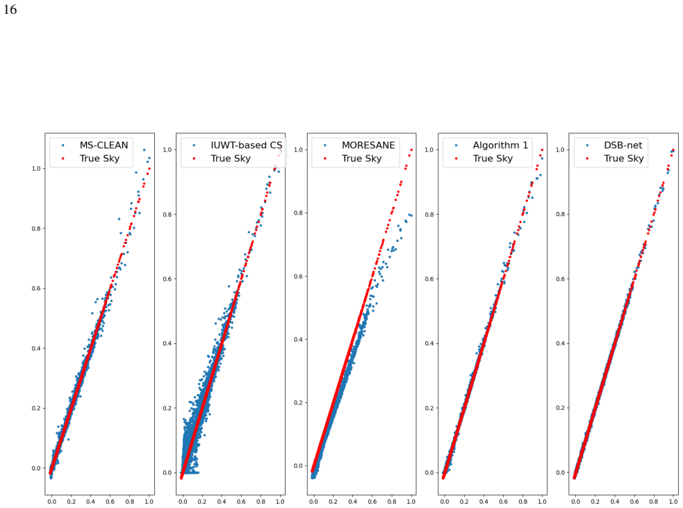
At the paper's center is the claim that a convolutional network can supply the sparsifying transform for compressive-sensing radio deconvolution while remaining inside the classical optimization loop rather than replacing it. The analysis path of the deep dictionary applies orthogonal filters per level followed by ReLU (read as the shrinkage operator) to produce multi-resolution sparse coefficients; the synthesis path reconstructs the image from coarse to fine. Inserted into split Bregman, the network's parameters and the reconstructed image are updated alternately until the $\ell_1$ and total-variation objective converges. In the reported simulations this yields DR = 2173 versus 48 for MS-CLEAN on M31 and DR = 32606 versus 331 on 3C 288, with the point-source experiment showing only a mild gain, indicating the method's strength is extended emission.
Load-bearing premise
The paper's load-bearing premise is that for radio interferometry the conditions of compressive sensing reduce to sparse representation — that the VLA u-v sampling and the learned dictionary are incoherent enough for $\ell_1$ recovery to be stable; if that incoherence does not hold, the reported gains could come from per-image fitting rather than from the CS guarantee.
Editorial extensions
If this is right
- Extended, low-surface-brightness sources that sit below the noise level become recoverable without a labeled training set, since the dictionary adapts to the data at hand.
- The same numerical machinery (split Bregman with $\ell_1$, TV, and a learned dictionary) transfers to other interferometers and to any linear inverse problem where a sparse prior is plausible.
- Because every network operation maps to a step of split Bregman, the reconstruction is auditable: one can check whether a given feature traces to the data-fidelity term, the TV term, or the dictionary.
- The point-source experiment shows the method's advantage is specific to extended structure: on point-like fields DSB-net's RMS is only about a third of MS-CLEAN's, so the practical use case is diffuse emission, not compact calibration sources.
- The reported run times mean a single $1024\times 1024$ DSB-net reconstruction takes roughly 4700 seconds on a modern GPU versus about 290 seconds for MS-CLEAN on CPU, so the gain in fidelity is bought with compute.
Reading between the lines
- If the sparsity-only simplification is accepted, then the real test of DSB-net is not image quality on one field but whether the learned dictionary stays incoherent with the u-v sampling operator across array configurations; a coherence audit would turn the empirical gain into a guarantee.
- The same design pattern — an overcomplete, data-adaptive dictionary inside an ADMM-style solver — could be applied to other ill-posed astronomical inversions where ground truth is unavailable, such as total-power short-spacing recovery, polarimetric imaging, or deconvolution of optical survey PSFs.
- Because the dictionary is learned per observation rather than pre-trained on a corpus, the method is naturally robust to source types not seen before; a wider test on real LOFAR or MeerKAT data would show whether that adaptation transfers beyond VLA simulations.
Signed reviews
Editorial analysis
A structured set of objections, weighed in public.
Referee Report
Summary. The paper proposes DSB-net, an unsupervised deconvolution method for radio interferometric imaging that integrates a learned 'deep dictionary' (implemented as a multi-resolution convolutional neural network) into a compressive-sensing split Bregman optimization framework. The authors argue that for radio interferometers the CS recovery conditions reduce to sparse representation, and they train the dictionary in an unsupervised, data-adaptive manner while alternating between image reconstruction and dictionary/parameter updates. The method is tested on simulated VLA observations of M31, 3C 288, and a point-source model, comparing against MS-CLEAN, IUWT-based CS, MORESANE, and a fixed-DWT version of the proposed algorithm. The headline results are RMS errors about 1% of MS-CLEAN's and dynamic ranges 45–100 times higher, with code made publicly available.
Significance. If the central numerical claims are established, the paper would present a substantial advance: an unsupervised, interpretable deep-learning deconvolution method that outperforms CLEAN-based and fixed-dictionary CS methods on extended, complex morphology sources, without requiring labeled training data. The method is clearly specified, the split Bregman formulation is a sound basis for integration with learned dictionaries, and the release of code is valuable. The qualitative error images suggest genuinely good reconstructions. However, the headline quantitative claim currently rests on residual-based metrics that may be inflated by in-sample fitting, and the theoretical CS justification is not verified for the learned dictionary or the specific array configurations used. These issues do not invalidate the method but require additional evidence before the performance claims can be accepted.
major comments (3)
- [Section 4, Eq. (12)–(13), Tables 1 and 3] The central numerical claim relies on metrics that measure data-fitting residuals, not accuracy against the known ground-truth sky. Eq. (12) defines 'rms error' as the RMS of the residual image, and Eq. (13) defines dynamic range as max(restored image) divided by that residual RMS. Because the deep dictionary and the Bregman parameters are learned on the same visibility data (Algorithm 2, Section 3.3), a sufficiently flexible model can drive residuals below the thermal noise floor and inflate DR even when the restored image contains artifacts. The only quantitative accuracy-vs-truth evidence is the qualitative model-absolute-error images in Figs. 4, 8, and 12; no numerical error-to-truth metric (e.g., normalized RMS of the model error, PSNR, or SSIM) is reported for any method. The authors should report such metrics for all methods, ideally also on a held-out sky model or a different noise realization, to support the headline 'RMS error about 1% of MS-CLEAN' and the 45–100x DR advantage. The overfitting test in Section 5 (reducing the number of base vectors to 6) is not conclusive because it still evaluates in-sample residuals on the same data.
- [Section 2.1] The claim that CS applicability for radio interferometry reduces to sparse representation alone is asserted from citations (Candes & Plan 2011; Wright & Ma 2022) and from generic Fourier incoherence arguments, but it is not verified for the actual problem setting. The measurement matrix in the experiments is a specific VLA uv-coverage (B or C configuration, with robust weighting), and the sparsifying dictionary is a learned, data-dependent CNN basis, not a fixed wavelet or Fourier basis. The coherence μ(Φ,Ψ) defined in Eq. (22) could be computed numerically for the learned dictionary and the actual sampling matrix; without such a check, the theoretical guarantee motivating Eq. (2) is not established. Please add an empirical coherence or RIP assessment, or explicitly frame the method as heuristic and temper the CS-theory justification accordingly.
- [Section 3.2, Eq. (9)] The symmetry loss L_symmetry = ||Ψ^T(Ψ(V_m)) – V_m||^2 applies the image-domain deep dictionary Ψ to the visibility data V_m, but the dictionary is intended to provide a sparse representation of the sky brightness image I in Eq. (4). It is not obvious why imposing symmetry on visibilities should produce a good sparsifying basis for images; the dictionary is never directly trained to reconstruct or sparsify I. The authors should either justify this design choice (e.g., by noting that V_m gridded on the same pixel grid approximates a linear transformation of I) or add a sparsity/symmetry term defined on the image domain.
minor comments (5)
- [Table 2] The table title contains a typo: 'MS-CEALN' should be 'MS-CLEAN'.
- [Table 2 and Section 4] The runtime comparison is not apples-to-apples: DSB-net runs on an RTX 4090 GPU while MS-CLEAN runs on a CPU. This should be stated prominently or the comparison should be made on the same hardware.
- [References, Introduction] The reference 'Högbom & Cornwell (1974)' is incorrect: Högbom's 1974 paper has a single author; Cornwell is associated with later CLEAN variants such as multi-scale CLEAN. Please correct the citation and the reference list entry.
- [Eq. (5)] In Eq. (5), 'such to' should be 'subject to'. Also, the ReLU notation in Eqs. (35)–(37) with two arguments is unconventional; ReLU(x) = max(x, 0) should be used consistently.
- [Section 5 and Abstract] The word 'fully interpretable' is stronger than what is demonstrated: the learned filters are not analyzed or visualized, and the dictionary update is a black-box optimizer. Consider softening this claim.
Assumptions & free parameters
free parameters (6)
- Initial Bregman weights mu0, lambda0, gamma0 =
40, 100, 1/(3 N_sigma) for DSB; 40, 1/(3 N_sigma), 1/N_sigma for fixed DWT
- Constraint weights alpha1, alpha2 =
0.001 and 0.01
- Decomposition level of deep dictionary =
5
- Filter size and number of filters per level =
5x5 and 25 per level
- Learning rate and optimizer =
Adam, 0.001 for DSB; 0.1 for fixed dictionary
- Convergence thresholds =
L_total = 0.7, L_fidelity = 1e-5, epsilon_d
assumptions (6)
- standard math Compressed sensing conditions (sparsity, incoherence, RIP) guarantee stable recovery of sparse signals.
- domain assumption For radio interferometric telescopes, CS applicability reduces to sparse representation; incoherence and RIP are assumed to hold for UV coverage.
- domain assumption The sky brightness can be sparsely represented in the learned deep dictionary.
- domain assumption Measurement noise is white Gaussian and calibration is perfect.
- ad hoc to paper The deep dictionary is a tight frame, Psi^T Psi approximately I, and filters are orthogonal per layer.
- standard math Split Bregman iteration converges for the alternating image and dictionary updates.
Cite this review
Pith. "Pith review of An Unsupervised Learning Method for Radio Interferometry Deconvolution." pith.science (2026). https://pith.science/paper/5WUODIGS
@misc{pith2026250504887,
  author       = {Pith},
  title        = {Pith review of: An Unsupervised Learning Method for Radio Interferometry Deconvolution},
  year         = {2026},
  howpublished = {\url{https://pith.science/paper/5WUODIGS}},
  note         = {Machine review of arXiv:2505.04887}
}
read the original abstract
Given the incomplete sampling of spatial frequencies by radio interferometers, achieving precise restoration of astrophysical information remains challenging. To address this ill-posed problem, compressive sensing(CS) provides a robust framework for stable and unique recovery of sky brightness distributions in noisy environments, contingent upon satisfying specific conditions. We explore the applicability of CS theory and find that for radio interferometric telescopes, the conditions can be simplified to sparse representation. {{Building on this insight, we develop a deep dictionary (realized through a convolutional neural network), which is designed to be multi-resolution and overcomplete, to achieve sparse representation and integrate it within the CS framework. The resulting method is a novel, fully interpretable unsupervised learning approach that combines}} the mathematical rigor of CS with the expressive power of deep neural networks, effectively bridging the gap between deep learning and classical dictionary methods. {{During the deconvolution process, the model image and the deep dictionary are updated alternatively.}} This approach enables efficient and accurate recovery of extended sources with complex morphologies from noisy measurements. Comparative analyses with state-of-the-art algorithms demonstrate the outstanding performance of our method, i.e., achieving a dynamic range (DR) nearly 45 to 100 times higher than that of multiscale CLEAN (MS-CLEAN).
Figures


Figures from the paper (9 more)




Reference graph
Works this paper leans on
-
[1]
, " * write output.state after.block = add.period write newline
ENTRY address archivePrefix author booktitle chapter doi edition editor eprint howpublished institution journal key month number organization pages publisher school series title misctitle type volume year version url label extra.label sort.label short.list INTEGERS output.state before.all mid.sentence after.sentence after.block FUNCTION init.state.consts ...
-
[2]
write newline
" write newline "" before.all 'output.state := FUNCTION format.url url empty "" new.block "" url * "" * if FUNCTION format.eprint eprint empty "" archivePrefix empty "" archivePrefix "arXiv" = new.block " " eprint * " " * new.block " " eprint * " " * if if if FUNCTION format.doi doi empty "" " " doi * " " * if FUNCTION format.pid doi empty eprint empty ur...
-
[3]
z Q . ,p C. ror lN, @
thebibliography [1] 20pt to REFERENCES 6pt =0pt -12pt 10pt plus 3pt =0pt =0pt =1pt plus 1pt =0pt =0pt -12pt =13pt plus 1pt =20pt =13pt plus 1pt \@M =10000 =-1.0em =0pt =0pt 0pt =0pt =1.0em @enumiv\@empty 10000 10000 `\.\@m \@noitemerr \@latex@warning Empty `thebibliography' environment \@ifnextchar \@reference \@latexerr Missing key on reference command E...
2021
-
[4]
2017, The Astronomical Journal, 153, 159, 10.3847/1538-3881/aa6302
Akiyama, K., Ikeda, S., Pleau, M., et al. 2017, The Astronomical Journal, 153, 159, 10.3847/1538-3881/aa6302
-
[5]
2010, Foundations and Trends® in Machine Learning, 3, 1, 10.1561/2200000016
Boyd, S. 2010, Foundations and Trends® in Machine Learning, 3, 1, 10.1561/2200000016
-
[6]
Cai, X., Pereyra, M., & McEwen, J. D. 2018, Monthly Notices of the Royal Astronomical Society, 480, 4170, 10.1093/mnras/sty2015
-
[7]
2008, IEEE Signal Processing Magazine, 25, 21, 10.1109/MSP.2007.914731
Candes, E., & Wakin, M. 2008, IEEE Signal Processing Magazine, 25, 21, 10.1109/MSP.2007.914731
arXiv 2008
-
[8]
Candes, E. J., & Plan, Y. 2011, IEEE Transactions on Information Theory, 57, 7235, 10.1109/TIT.2011.2161794
Show all 46 references
-
[9]
J., Romberg, J
Candès, E. J., Romberg, J. K., & Tao, T. 2006, Communications on Pure and Applied Mathematics, 59, 1207, 10.1002/cpa.20124
2006 doi
-
[10]
E., McEwen, J
Carrillo, R. E., McEwen, J. D., & Wiaux, Y. 2012, Monthly Notices of the Royal Astronomical Society, 426, 1223, 10.1111/j.1365-2966.2012.21605.x
2012
-
[11]
N., Girard, J
Chiche, B. N., Girard, J. N., Frontera-Pons, J., Woiselle, A., & Starck, J.-L. 2023, Astronomy & Astrophysics, 675, A116, 10.1051/0004-6361/202245013
2023 doi
-
[12]
2019, in Inverse Acoustic and Electromagnetic Scattering Theory , Vol
Colton, D., & Kress, R. 2019, in Inverse Acoustic and Electromagnetic Scattering Theory , Vol. 93 (Cham: Springer International Publishing), 111--136, 10.1007/978-3-030-30351-8_4
2019 doi
-
[13]
Cornwell, T. J. 2008, IEEE Journal of Selected Topics in Signal Processing, 2, 793, 10.1109/JSTSP.2008.2006388
2008
-
[14]
2015, Astronomy & Astrophysics, 576, A7, 10.1051/0004-6361/201424602
Dabbech, A., Ferrari, C., Mary, D., et al. 2015, Astronomy & Astrophysics, 576, A7, 10.1051/0004-6361/201424602
2015 doi
-
[15]
2006 a , IEEE Transactions on Information Theory, 52, 1289, 10.1109/TIT.2006.871582
Donoho, D. 2006 a , IEEE Transactions on Information Theory, 52, 1289, 10.1109/TIT.2006.871582
2006
-
[16]
Donoho, D. L. 2006 b , Communications on Pure and Applied Mathematics, 59, 907, 10.1002/cpa.20131
2006 doi
-
[17]
2010, Sparse and redundant representations: from theory to applications in signal and image processing (New York: Springer)
Elad, M. 2010, Sparse and redundant representations: from theory to applications in signal and image processing (New York: Springer)
2010
-
[18]
2013, A Mathematical Introduction to Compressive Sensing , Applied and Numerical Harmonic Analysis (New York, NY: Springer New York), 10.1007/978-0-8176-4948-7
Foucart, S., & Rauhut, H. 2013, A Mathematical Introduction to Compressive Sensing , Applied and Numerical Harmonic Analysis (New York, NY: Springer New York), 10.1007/978-0-8176-4948-7
2013 doi
-
[19]
N., Starck, J
Garsden, H., Girard, J. N., Starck, J. L., et al. 2015, Astronomy & Astrophysics, 575, A90, 10.1051/0004-6361/201424504
2015 doi
-
[20]
2012, Image Processing On Line, 2, 158, 10.5201/ipol.2012.g-tvdc
Getreuer, P. 2012, Image Processing On Line, 2, 158, 10.5201/ipol.2012.g-tvdc
2012 doi
-
[21]
2023, Astronomy & Astrophysics, 677, A167, 10.1051/0004-6361/202347073
Geyer, F., Schmidt, K., Kummer, J., et al. 2023, Astronomy & Astrophysics, 677, A167, 10.1051/0004-6361/202347073
2023 doi
-
[22]
2009, SIAM Journal on Imaging Sciences, 2, 323, 10.1137/080725891
Goldstein, T., & Osher, S. 2009, SIAM Journal on Imaging Sciences, 2, 323, 10.1137/080725891
2009 doi
-
[23]
2020, Proceedings of the AAAI Conference on Artificial Intelligence, 34, 10933, 10.1609/aaai.v34i07.6726
Han, X., Wu, B., Shou, Z., et al. 2020, Proceedings of the AAAI Conference on Artificial Intelligence, 34, 10933, 10.1609/aaai.v34i07.6726
2020 doi
-
[24]
Hastie, T., Tibshirani, R., & Friedman, J. H. 2009, The elements of statistical learning: data mining, inference, and prediction, 2nd edn., Springer series in statistics (New York, NY: Springer)
2009
-
[25]
A., & Cornwell, T
H \"o gbom, J. A., & Cornwell, T. J. 1974, Astronomy and Astrophysics, 500, 55. https://api.semanticscholar.org/CorpusID:116934453
1974
-
[26]
2022, IEEE Access, 10, 69741, 10.1109/ACCESS.2022.3185621
Kim, T., & Yun, S.-Y. 2022, IEEE Access, 10, 69741, 10.1109/ACCESS.2022.3185621
2022
-
[27]
2015, Nature, 521, 436, 10.1038/nature14539
LeCun, Y., Bengio, Y., & Hinton, G. 2015, Nature, 521, 436, 10.1038/nature14539
2015 doi
-
[28]
J., & De Hoog, F
Li, F., Cornwell, T. J., & De Hoog, F. 2011, Astronomy & Astrophysics, 528, A31, 10.1051/0004-6361/201015045
2011 doi
-
[29]
I., Mars, M., Price, M
Liaudat, T. I., Mars, M., Price, M. A., et al. 2024, RAS Techniques and Instruments, 3, 505, 10.1093/rasti/rzae030
2024 doi
-
[30]
Mallat, S. G. 2009, A wavelet tour of signal processing: the sparse way, 3rd edn. (Amsterdam ; Boston: Elsevier/Academic Press)
2009
-
[31]
Müller, H., & Lobanov, A. P. 2022, Astronomy & Astrophysics, 666, A137, 10.1051/0004-6361/202243244
2022 doi
-
[32]
N., et al
Nammour, F., Akhaury, U., Girard, J. N., et al. 2022, Astronomy & Astrophysics, 663, A69, 10.1051/0004-6361/202142626
2022 doi
-
[33]
2017, The Journal of Machine Learning Research, 18, 2887
Papyan, V., Romano, Y., & Elad, M. 2017, The Journal of Machine Learning Research, 18, 2887
2017
-
[34]
M., & Elad, M
Rubinstein, R., Bruckstein, A. M., & Elad, M. 2010, Proceedings of the IEEE, 98, 1045, 10.1109/JPROC.2010.2040551
2010
-
[35]
2022, Astronomy & Astrophysics, 664, A134, 10.1051/0004-6361/202142113
Schmidt, K., Geyer, F., Fröse, S., et al. 2022, Astronomy & Astrophysics, 664, A134, 10.1051/0004-6361/202142113
2022 doi
-
[36]
2021, Compressive Sensing , Colóquios Brasileiros de Matemática (Rio de Janeiro, RJ: Associação Instituto Nacional de Matemática Pura e Aplicada)
Schulz, A. 2021, Compressive Sensing , Colóquios Brasileiros de Matemática (Rio de Janeiro, RJ: Associação Instituto Nacional de Matemática Pura e Aplicada)
2021
-
[37]
Schwab, F. R. 1984, The Astronomical Journal, 89, 1076, 10.1086/113605
1984 doi
-
[38]
Starck, J.-L., Murtagh, F., & Fadili, J. M. 2010, Sparse image and signal processing: wavelets, curvelets, morphological diversity (Cambridge ; New York: Cambridge University Press)
2010
-
[39]
Taylor, G., Carilli, C., Perley, R., & (U.S.), N. R. A. O. 1999, Synthesis imaging in radio astronomy II : a collection of lectures from the Sixth NRAO / NMIMT Synthesis Imaging Summer School held at Socorro , New Mexico , USA , 17-23 June , 1998, Astronomical Society of the P...
1999
-
[40]
2022, Monthly Notices of the Royal Astronomical Society, 518, 604, 10.1093/mnras/stac2672
Terris, M., Dabbech, A., Tang, C., & Wiaux, Y. 2022, Monthly Notices of the Royal Astronomical Society, 518, 604, 10.1093/mnras/stac2672
2022 doi
-
[41]
R., Moran, J
Thompson, A. R., Moran, J. M., & Swenson, G. W. 2017, Interferometry and Synthesis in Radio Astronomy , Astronomy and Astrophysics Library (Cham: Springer International Publishing), 10.1007/978-3-319-44431-4
2017 doi
-
[42]
2020, An introduction to compressed sensing (Philadelphia: SIAM, Society for Industrial and Applied Mathematics)
Vidyasagar, M. 2020, An introduction to compressed sensing (Philadelphia: SIAM, Society for Industrial and Applied Mathematics)
2020
-
[43]
2022, High- Dimensional Data Analysis with Low - Dimensional Models : Principles , Computation , and Applications , 1st edn
Wright, J., & Ma, Y. 2022, High- Dimensional Data Analysis with Low - Dimensional Models : Principles , Computation , and Applications , 1st edn. (Cambridge University Press), 10.1017/9781108779302
2022 doi
-
[44]
2021, IEEE Transactions on Medical Imaging, 40, 1329, 10.1109/TMI.2021.3054167
Xiang, J., Dong, Y., & Yang, Y. 2021, IEEE Transactions on Medical Imaging, 40, 1329, 10.1109/TMI.2021.3054167
2021
- [45]
-
[46]
2018, in 2018 IEEE / CVF Conference on Computer Vision and Pattern Recognition (Salt Lake City, UT: IEEE), 1828--1837, 10.1109/CVPR.2018.00196
Zhang, J., & Ghanem, B. 2018, in 2018 IEEE / CVF Conference on Computer Vision and Pattern Recognition (Salt Lake City, UT: IEEE), 1828--1837, 10.1109/CVPR.2018.00196
2018
Reviewed August 15, 2026 · model on record in the stance chip above.
Discussion (0). Continue with ORCID to comment.