REVIEW 3 major objections 6 minor 13 references
A new methodology to decompose a parametric domain using reduced order data manifold in machine learning
T0 review · 3 major / 6 minor · reviewed 2026-08-15 · deepseek-v4-flash
Pith's one-line read On a harmonic-transport benchmark, decomposing the parameter domain through a stretched one-dimensional manifold cuts high-dimensional surrogate error by 22%.
desk verdict The decomposition idea is genuinely novel, but the inverse-projection theorem is wrong and the headline 22% gain comes from a baseline tuned with different hyperparameters on a single 200-sample test set. read the letter →
The pith
A machine-rendered reading of the paper's core claim, the machinery that carries it, and where it could break.
The reading
What carries the argument
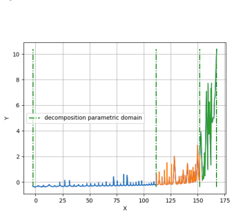
The load-bearing object is the stretched 1-manifold: a curve obtained by iPCA-reducing both inputs and outputs to one dimension, tracing the connected curve of the point cloud with ball-pivoting triangulation, and unfolding it segment-by-segment with mirror functions of the form φ_j(˜x, ˜y)=(2˜x_j−˜x, ˜y) at each turning point. This produces a functional scalar curve on which LISSDA applies a line-similarity threshold to carve out branched parametric domains. The inverse projectors—the pseudo-inverse composition of Theorem 2.2 and the component-complement minimization of Theorem 2.3—are what allow predictions made in the latent curve to be mapped back to the original output space.
What would settle it
Take any training output point, compute its one-dimensional iPCA coordinate, then reconstruct it with the pseudo-inverse projector. If the relative reconstruction error is not near zero—for example, larger than a few percent on the high-dimensional harmonic-transport outputs—then the inverse step is only approximate and the latent-space interpolation results must be reinterpreted. Since the outputs live in 2048 dimensions and the manifold is reduced to one coordinate, the discarded complement should contain most of the variance.
Extended reading notes
Core claim
The paper's central claim is that a high-dimensional parametric data manifold can be reduced to a one-dimensional curve in a way that preserves enough structure to partition the parameter domain into meaningful subdomains. Iterative PCA sequentially removes the least-informative singular-vector columns so each step keeps the maximum explained variance; applying it to inputs and outputs yields a 1-manifold. A mirror-function stretching unfolds this curve into a functional form, and LISSDA segments it into quasi-linear pieces. Local multilayer perceptrons trained on the original-data subdomains defined by these pieces outperform a single global MLP. In the high-dimensional benchmark, the weighted decomposed-domain error drops from 0.58 to 0.45 mean relative error, a 22% improvement, and in the low-dimensional case the iPCA-based latent interpolation beats the PCA-based one by about a factor of two (1.04 versus 2.05).
Load-bearing premise
The load-bearing premise is that a point's position on the one-dimensional curve determines the full high-dimensional output exactly, so projecting back from the curve recovers all the information; the proof of the inverse step assumes the discarded dimensions carry no information, which is not true when reducing to one dimension.
Editorial extensions
If this is right
- On the harmonic-transport benchmark, replacing a single global MLP with MLPs trained on LISSDA subdomains reduces mean relative error from 0.58 to 0.45 for high-dimensional outputs, a 22% drop.
- Using iPCA rather than classical PCA to build the 1-manifold roughly halves the interpolation error in the low-dimensional-output case (1.04 versus 2.05).
- The inverse projectors let latent-space predictions be mapped back to original outputs, making the stretched manifold usable as a surrogate even when outputs are not scalars.
- The decomposition is discovered from data, so it can expose parameter regimes without prior physical knowledge of where regime boundaries lie.
Reading between the lines
- Our inference: the 22% improvement may come mostly from local modeling rather than from iPCA itself; a baseline that clusters the original parameter space into the same number of subdomains would isolate the contribution of the stretched-manifold geometry.
- Our inference: because the pseudo-inverse reconstruction is approximate for one-dimensional reductions, the latent interpolation results likely under-report the true error, while the MLP results, which do not rely on inverse projection, are the safer evidence for the method.
- Our inference: the line-similarity threshold γ controls the number of subdomains, but the paper gives no rule for choosing it; a testable extension would tie γ to a validation-error plateau so the decomposition adapts automatically.
- Our inference: mirror-function stretching turns a folded curve into a function, but it may create artificial discontinuities at turning points; applying the method to data with known regime boundaries, such as phase transitions, would test whether segment boundaries align with physical transitions.
Signed reviews
Editorial analysis
A structured set of objections, weighed in public.
Referee Report
Summary. The paper proposes a methodology for parametric domain decomposition based on a reduced-order data manifold. The main components are: iterative PCA (iPCA) to reduce high-dimensional data to a 1-manifold, two inverse projectors (pseudo-inverse and component-complement), a stretching procedure (global mirror function) to turn the 1-manifold into a single-valued curve, and a line-similarity segmentation algorithm (LISSDA) that decomposes the stretched manifold into subdomains. The methods are tested on a harmonic transport problem with scalar and high-dimensional outputs, comparing the proposed pipeline with classical PCA, UMAP, and full-domain multilayer perceptrons (MLPs). The central claim is that the stretched-manifold decomposition improves surrogate-model accuracy, with a headline result of 0.45 mean relative error for the weighted decomposed-domain MLP versus 0.58 for the full-domain MLP in the high-dimensional output case.
Significance. If the claims hold, the idea of using the geometry of a reduced-order data manifold to inform parametric domain decomposition is a useful contribution to surrogate modeling, particularly in small-data regimes. The paper clearly describes the experimental setting (harmonic transport problem) and provides comparisons against several baselines. The authors also state the limitation that the methodology should be tested on nonlinear behaviors, which is commendable. However, the main quantitative claim is not yet reliable because of uncontrolled hyperparameter choices and missing uncertainty estimates, and a central theoretical claim (Theorem 2.2) is demonstrably overclaimed. The manuscript does not provide code or data, which limits reproducibility.
major comments (3)
- [§2.1.1, Theorem 2.2 / Appendix 1] The proof of Theorem 2.2 in Appendix 1 derives X_{j-1} = X_j F_j by omitting the complement term X_j^c V_j^{cT} that the authors themselves introduce in Theorem 2.3. Because iPCA reduces the data to a 1-manifold by discarding that complement, the pseudo-inverse reconstruction is exact only when the data lies in the retained subspace, which is not the case here. Thus the statement that X' = X'_k π_k^{-1} is an exact inverse is incorrect, and the pseudo-inverse rows of Table 3 overstate the accuracy of the inversion strategy.
- [§3.3.2, Table 3] The comparison between the full-domain MLP and the decomposed-domain MLPs is not made on equal footing: the full-domain MLP uses learning rate 1.4e-3 and batch size 50, while the two decomposed-domain MLPs use learning rates 4.72e-5 and 4.72e-6 with batch size 20, with the text stating only that "a good learning rate" was chosen per model. All results are reported on a single 200-sample test set with no repeated seeds or confidence intervals. Given the reported test variances of 0.30–0.57, the 0.13 difference in mean relative error between the weighted domain (0.45) and the full domain (0.58) is within plausible sampling noise, so the claimed 22% improvement is not established.
- [§2.2.2, Theorem 2.4] The global mirror function theorem asserts that any connected continuous 1-manifold can be transformed into a single-valued function, but the proof is an induction sketch that assumes turning points are well-defined and that repeated reflections at turning points cannot create new folds, self-intersections, or non-functional regions. In addition, the extraction of the connected curve by ball pivoting and "lowest edge" is heuristic and is not validated on noisy or uneven point clouds. Since LISSDA and the parametric decomposition in §2.3 operate entirely on the stretched manifold, the validity of the proposed decomposition depends on these unproven assumptions.
minor comments (6)
- [Abstract] The phrase "iterative principle component analysis" should be "iterative principal component analysis."
- [§3.1] "Chebeshev" and "polynimial" are misspelled; these should be "Chebyshev" and "polynomial."
- [§3.3.2 and Table 3] The text refers to "the third case" and to "the first and second cases," but only two cases are presented; the case numbering should be corrected.
- [§2.4] Because the data are stated to be standardized before computing the latent representation, the reconstruction formula ŷ_train = π_y^{-1}∘g∘Φ|_x∘π_x(x_train) does not explicitly include an unstandardization step; the paper should clarify how predictions are mapped back to the original output scale.
- [Appendix 2, Algorithm 2] The control flow in LISSDA is unclear: when LISP returns ok=True, the code sets L←C and C←empty, discarding the list L returned by LISP; the pseudo-code should be revised for clarity.
- [§3.3.1] The statement that the iPCA manifold error is "closed to 100% better" than the PCA manifold error is imprecise; the reported mean errors of 1.04 and 2.05 correspond to roughly a 49% reduction, not 100%.
Circularity Check
No significant circularity: the method is an externally benchmarked supervised pipeline; no self-citation chain or fit-renamed-as-prediction.
full rationale
The paper's central claims are validated by comparisons against independently implemented baselines (classical PCA, UMAP, and full-domain MLPs) on held-out test sets generated from the harmonic transport problem. The iPCA inverse projectors are presented as mathematical constructions with proofs; even if Theorem 2.2's pseudo-inverse reconstruction is questionable when the kept subspace is only one-dimensional, that is a correctness or approximation issue, not a circular derivation, because the inverse projectors are not defined in terms of the benchmark errors they are used to explain. The stretched 1-manifold and LISSDA decomposition are constructed from training data (X,Y) and are then applied to test inputs through nearest-training-point classification, so the test predictions are not obtained by reusing the test outputs. The gamma threshold and MLP learning rates/batch sizes are user-chosen hyperparameters; the paper reports them explicitly and does not rename a fitted value as a prediction, so any concern about tuning or unequal comparison of baselines is a statistical or benchmarking concern rather than circularity. There are no load-bearing self-citations: the reference list contains no prior work by the present authors, and no uniqueness theorem is imported from the authors' own earlier papers. The derivation chain is self-contained and externally benchmarked, so no circular step can be exhibited from the paper's equations or citations.
Assumptions & free parameters
free parameters (3)
- gamma (line similarity threshold) =
gamma=4 (case 1), gamma=2 (case 2), gamma=1.5 (appendix case)
- MLP per-domain hyperparameters =
learning rates 5.33e-6 to 6.2e-9, batch sizes 5-50, 1-2 hidden layers with 10-3680 nodes
- epsilon in LISP algorithm =
unspecified
assumptions (5)
- domain assumption The parametric domain X is open and the data manifold is a continuous multivariable vectorial function.
- ad hoc to paper The iterative mirror function unfolding (Theorem 2.4) maps any connected continuous 1-manifold to a single-valued function.
- ad hoc to paper The ball-pivoting algorithm applied to the 1-manifold point cloud yields the correct connectivity, and the 'lowest edge' extraction produces the true connected curve.
- standard math Moore-Penrose pseudo-inverse properties as used for the inverse projector.
- domain assumption For a test sample, the nearest training neighbor determines the correct BPD and mirror function.
Cite this review
Pith. "Pith review of A new methodology to decompose a parametric domain using reduced order data manifold in machine learning." pith.science (2026). https://pith.science/paper/XBU65AOO
@misc{pith2026250508497,
  author       = {Pith},
  title        = {Pith review of: A new methodology to decompose a parametric domain using reduced order data manifold in machine learning},
  year         = {2026},
  howpublished = {\url{https://pith.science/paper/XBU65AOO}},
  note         = {Machine review of arXiv:2505.08497}
}
read the original abstract
We propose a new methodology for parametric domain decomposition using iterative principal component analysis. Starting with iterative principle component analysis, the high dimension manifold is reduced to the lower dimension manifold. Moreover, two approaches are developed to reconstruct the inverse projector to project from the lower data component to the original one. Afterward, we provide a detailed strategy to decompose the parametric domain based on the low dimension manifold. Finally, numerical examples of harmonic transport problem are given to illustrate the efficiency and effectiveness of the proposed method comparing to the classical meta-models such as neural networks.
Figures


Figures from the paper (2 more)

Reference graph
Works this paper leans on
-
[1]
Hierarchical mixtures of experts and the em algorithm.Neural computation, 6(2):181–214, 1994
Michael I Jordan and Robert A Jacobs. Hierarchical mixtures of experts and the em algorithm.Neural computation, 6(2):181–214, 1994
1994
-
[2]
A domain decomposition method for fast manifold learning
Zhenyue Zhang and Hongyuan Zha. A domain decomposition method for fast manifold learning. Advances in Neural Information Processing Systems, 18, 2005
work page 2005
-
[3]
Acceleration techniques for reduced-order models based on proper orthogonal decomposition
Paul GA Cizmas, Brian R Richardson, Thomas A Brenner, Thomas J O’Brien, and Ronald W Breault. Acceleration techniques for reduced-order models based on proper orthogonal decomposition. Journal of Computational Physics, 227(16):7791–7812, 2008
work page 2008
-
[4]
Marc Sauget, Rémy Laurent, Julien Henriet, Michel Salomon, Régine Gschwind, Sylvain Contassot-Vivier, Libor Makovicka, and Charles Soussen. Efficient domain decomposition for a neural network learning algorithm, used for the dose evaluation in external radiotherapy. In International Conference on Artificial Neural Networks, pages 261–266. Springer, 2010
work page 2010
-
[5]
Bernard Haasdonk, Markus Dihlmann, and Mario Ohlberger. A training set and multiple bases generation approach for parameterized model reduction based on adaptive grids in parameter space. Mathematical and Computer Modelling of Dynamical Systems, 17(4):423–442, 2011
work page 2011
-
[6]
Domain-decomposed bayesian inversion based on local karhunen-loève expansions
Zhihang Xu, Qifeng Liao, and Jinglai Li. Domain-decomposed bayesian inversion based on local karhunen-loève expansions. Journal of Computational Physics, page 112856, 2024
work page 2024
-
[7]
Principal components analysis (pca)
Steven M Holland. Principal components analysis (pca). Department of Geology, University of Georgia, Athens, GA, 30602:2501, 2008
work page 2008
-
[8]
The moore–penrose pseudoinverse: A tutorial review of the theory
João Carlos Alves Barata and Mahir Saleh Hussein. The moore–penrose pseudoinverse: A tutorial review of the theory. Brazilian Journal of Physics, 42:146–165, 2012
2012
Show all 13 references
-
[9]
The ball-pivoting algorithm for surface reconstruction
Fausto Bernardini, Joshua Mittleman, Holly Rushmeier, Cláudio Silva, and Gabriel Taubin. The ball-pivoting algorithm for surface reconstruction. IEEE transactions on visualization and computer graphics, 5(4):349–359, 1999
1999
-
[10]
Mathematical analysis of goldstein’s model for time-harmonic acoustics in flows
Antoine Bensalah, Patrick Joly, and Jean-Francois Mercier. Mathematical analysis of goldstein’s model for time-harmonic acoustics in flows. ESAIM: Mathematical Modelling and Numerical Analysis, 56(2):451–483, 2022
2022
-
[11]
An adaptive sampling strategy for kriging metamodel based on delaunay triangulation and topsis
Ping Jiang, Yahui Zhang, Qi Zhou, Xinyu Shao, Jiexiang Hu, and Leshi Shu. An adaptive sampling strategy for kriging metamodel based on delaunay triangulation and topsis. Applied Intelligence, 48:1644–1656, 2018
2018
-
[12]
Umap: Uniform manifold approximation and projection for dimension reduction
Leland McInnes, John Healy, and James Melville. Umap: Uniform manifold approximation and projection for dimension reduction. arXiv preprint arXiv:1802.03426, 2018
2018 arXiv
-
[13]
https://www.irt-systemx.fr/projets/hsa/
Irt systemx. https://www.irt-systemx.fr/projets/hsa/. Accessed: 2024-05-20. 11 Theoretical study of performances of numerical and automatic differentiation physical informed neural network APPENDIX 1: PROOF OF THEOREMS Proof of Theorem 2.1. Given that the original data X = X0 ...
2024
Reviewed August 15, 2026 · model on record in the stance chip above.
Discussion (0). Continue with ORCID to comment.