Assumption-lean weak limits and tests for two-stage adaptive experiments
Pith reviewed 2026-05-22 13:58 UTC · model grok-4.3
The pith
Two-stage adaptive experiments admit weak limits for weighted inverse probability weighted estimators under weaker assumptions.
A machine-rendered reading of the paper's core claim, the machinery that carries it, and where it could break.
Core claim
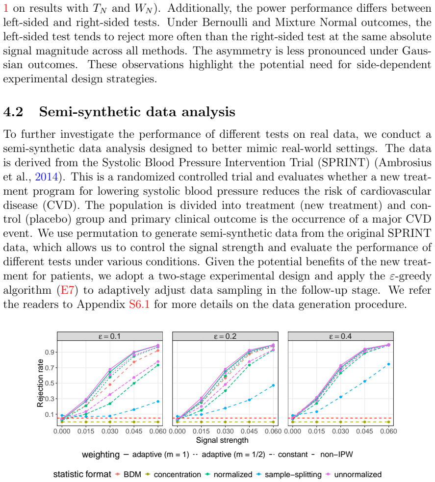
In two-stage adaptive experimental designs the weighted inverse probability weighted estimators of mean outcomes and differences possess weak limits whose form depends on the underlying signal regime; these limits are obtained under weaker assumptions than prior results and thereby unify previously separate findings for different adaptive schemes.
What carries the argument
Weighted inverse probability weighted (WIPW) estimators, which reweight each observation by the inverse of its realized sampling probability across the two stages so that expectations remain consistent despite data-dependent adaptation.
If this is right
- Hypothesis testing remains valid even when the limiting distribution is non-normal by using critical values drawn from the simulation procedure.
- Convergence rates in bounded-Lipschitz distance make explicit the tension between more aggressive exploitation in the second stage and the stability of subsequent inference.
- The same weak-limit statements cover both batched bandit designs and subgroup enrichment experiments under the two-stage structure.
- Results that previously appeared only in isolated signal regimes now appear as special cases of a single set of theorems.
Where Pith is reading between the lines
- The simulation method for critical values could be reused in other adaptive procedures whose limits are also non-normal.
- If similar measurability conditions can be verified, the weak-convergence arguments might extend to designs with three or more stages.
- Experimenters could deliberately vary first-stage signal strength to observe the predicted change in limiting behavior and thereby test the phase-transition claim directly.
Load-bearing premise
The design consists of exactly two stages and the second-stage sampling probabilities depend on first-stage data in a measurable way that keeps the weighted inverse probability weights well-defined for weak convergence arguments.
What would settle it
In a controlled two-stage adaptive experiment with known signal strength, if the empirical distribution of the WIPW estimator fails to approach the predicted weak limit or to exhibit the claimed phase transition when signal strength crosses the relevant threshold, the results would be falsified.
Figures


read the original abstract
Adaptive experiments are becoming increasingly popular in real-world applications for effectively maximizing in-sample welfare and efficiency by data-driven sampling. Despite their growing prevalence, however, the statistical foundations for valid inference in such settings remain underdeveloped. Focusing on two-stage adaptive experimental designs, we address this gap by deriving new weak convergence results for mean outcomes and their differences. In particular, our results apply to a broad class of estimators, the weighted inverse probability weighted (WIPW) estimators. In contrast to prior works, our results require significantly weaker assumptions and sharply characterize phase transitions in limiting behavior across different signal regimes. Through this common lens, our general results unify previously fragmented results under the two-stage setup. We further establish quantitative convergence rates in bounded-Lipschitz distance that reveal the fundamental trade-off between exploitation and inferential stability. To address the challenge of potential non-normal limits in conducting inference, we propose a computationally efficient and provably valid simulation-based method for obtaining critical values of the non-normal limiting distributions under the null, enabling practical hypothesis testing. Our results and approaches are sufficiently general to accommodate various adaptive experimental designs, including batched bandit and subgroup enrichment experiments. Simulations and semi-synthetic studies demonstrate the practical value of our approach and reveal that neither normality-based nor non-normality-based testing methods uniformly dominate in power; the relative advantage depends on the structure of the outcome distribution.
Editorial analysis
A structured set of objections, weighed in public.
Referee Report
Summary. The paper derives new weak convergence results for weighted inverse probability weighted (WIPW) estimators in two-stage adaptive experimental designs. It claims these results hold under significantly weaker assumptions than prior work, specifically allowing second-stage sampling probabilities to depend on first-stage data in a measurable way. The manuscript sharply characterizes phase transitions in limiting behavior (normal versus non-normal) across different signal regimes, provides quantitative convergence rates in bounded-Lipschitz distance, unifies previously fragmented results, and proposes a simulation-based method for obtaining critical values under non-normal limits to facilitate hypothesis testing. The results are illustrated with applications to batched bandit and subgroup enrichment experiments, supported by simulations and semi-synthetic studies.
Significance. Should the central claims hold, this manuscript would represent a significant advance in the statistical foundations for inference in adaptive experiments by relaxing key assumptions and providing a unified framework for handling different limiting regimes. The quantitative rates and the practical simulation method for non-normal cases are particularly valuable for applied researchers designing adaptive studies. The unification across designs like bandits and enrichment experiments broadens the impact.
major comments (2)
- Abstract and the statement of the main weak-convergence theorem: The central claim of 'significantly weaker assumptions' rests on allowing the second-stage sampling probabilities to depend on first-stage data only in a measurable way. However, this condition alone does not obviously preclude discontinuities in the adaptation map or sampling probabilities that can be arbitrarily close to zero on sets of positive measure. Such cases could introduce additional bias or variance terms that shift the phase-transition thresholds between normal and non-normal limits, undermining the 'sharply characterize' assertion. The proof must explicitly control these issues to support the claimed rates in bounded-Lipschitz distance.
- Section 4 on the simulation method: The proposed simulation procedure is presented as provably valid for obtaining critical values under non-normal limits. It is unclear whether the method remains valid uniformly across the signal regimes identified in the phase-transition analysis, particularly near the boundary where the limiting distribution changes. An explicit verification or additional assumption ensuring the simulation approximates the correct null distribution in all regimes would be required.
minor comments (2)
- The notation for the weighted inverse probability weights could be introduced more explicitly in the setup section to distinguish it clearly from standard IPW estimators.
- In the simulation studies, the description of how the outcome distributions vary across the different signal regimes is somewhat terse and would benefit from a short table summarizing the parameters used.
Simulated Author's Rebuttal
We thank the referee for the careful reading and constructive comments. We address each major comment below and indicate the revisions we will make to strengthen the manuscript.
read point-by-point responses
-
Referee: Abstract and the statement of the main weak-convergence theorem: The central claim of 'significantly weaker assumptions' rests on allowing the second-stage sampling probabilities to depend on first-stage data only in a measurable way. However, this condition alone does not obviously preclude discontinuities in the adaptation map or sampling probabilities that can be arbitrarily close to zero on sets of positive measure. Such cases could introduce additional bias or variance terms that shift the phase-transition thresholds between normal and non-normal limits, undermining the 'sharply characterize' assertion. The proof must explicitly control these issues to support the claimed rates in bounded-Lipschitz distance.
Authors: The referee correctly notes that measurability alone permits discontinuous adaptation maps and sampling probabilities that may approach zero. Our proof proceeds by conditioning on the first-stage sigma-field, under which the second-stage probabilities are non-random; the weak convergence is then obtained conditionally and integrated. The bounded-Lipschitz metric is used precisely because it is insensitive to discontinuities of the adaptation map. The phase-transition thresholds are expressed in terms of the realized conditional variances of the WIPW terms, so that any inflation of variance due to small sampling probabilities automatically shifts the threshold; no additional bias terms arise because the weights are exactly the inverse of the (measurable) probabilities. We will add a clarifying paragraph in the proof of the main theorem and a remark after the statement of the phase-transition result to make this explicit. revision: partial
-
Referee: Section 4 on the simulation method: The proposed simulation procedure is presented as provably valid for obtaining critical values under non-normal limits. It is unclear whether the method remains valid uniformly across the signal regimes identified in the phase-transition analysis, particularly near the boundary where the limiting distribution changes. An explicit verification or additional assumption ensuring the simulation approximates the correct null distribution in all regimes would be required.
Authors: We agree that uniformity across regimes, especially at the phase-transition boundary, needs explicit verification. The simulation draws from the estimated limiting random variable whose distribution is continuous in the signal-strength parameter; at the boundary the non-normal limit collapses to a Gaussian, so the simulated critical values converge to the normal quantiles. We will insert a new proposition establishing that the Kolmogorov distance between the simulated and true limiting distributions is bounded uniformly on compact sets of signal strengths that straddle the transition point, thereby confirming validity without extra assumptions. revision: yes
Circularity Check
No significant circularity; derivations rely on standard weak-convergence tools
full rationale
The paper applies standard weak-convergence arguments and measurability conditions to WIPW estimators in two-stage designs, deriving limits and phase transitions directly from the probabilistic structure without reducing any claimed result to a fitted parameter or self-citation that defines the target quantity. The unification of prior results occurs by embedding them in the same general framework rather than by re-expressing the new limits in terms of the inputs. Simulations are described as an independent computational procedure for critical values, and no load-bearing step equates a prediction to its own construction.
Axiom & Free-Parameter Ledger
axioms (1)
- domain assumption The experiment proceeds in exactly two stages, with second-stage sampling probabilities depending on first-stage observations in a way that keeps the inverse-probability weights well-defined.
Lean theorems connected to this paper
-
IndisputableMonolith/Foundation/RealityFromDistinction.leanreality_from_one_distinction unclear?
unclearRelation between the paper passage and the cited Recognition theorem.
Theorem 1 (Weak convergence) ... Assumptions 1-4 ... phase transition ... c = -∞ yields Gaussian limit while c ∈ (-∞,0] yields non-normal limits
-
IndisputableMonolith/Cost/FunctionalEquation.leanwashburn_uniqueness_aczel unclear?
unclearRelation between the paper passage and the cited Recognition theorem.
quantitative convergence rates in bounded-Lipschitz distance ... clipping rate l_N
What do these tags mean?
- matches
- The paper's claim is directly supported by a theorem in the formal canon.
- supports
- The theorem supports part of the paper's argument, but the paper may add assumptions or extra steps.
- extends
- The paper goes beyond the formal theorem; the theorem is a base layer rather than the whole result.
- uses
- The paper appears to rely on the theorem as machinery.
- contradicts
- The paper's claim conflicts with a theorem or certificate in the canon.
- unclear
- Pith found a possible connection, but the passage is too broad, indirect, or ambiguous to say the theorem truly supports the claim.
Reference graph
Works this paper leans on
-
[1]
First stage sampling: Sample S(b) 1 ∼ N(0, I2) and let ˜A(1,b) = ( ˆΣ(1))1/2S(b) 1 , where ˆΣ(1) = ( ˆCov (1) )2×2
-
[2]
Second stage sampling: Sample S(b) 2 ∼ N(0, I2) and let ˜A(2,b) = ( ˆΣ(2,b))1/2S(b) 2 , where ˆΣ(2,b) = ( ˆCov (2) ( ˜A(1,b)))2×2
-
[3]
Weighting procedure: Compute weights ˆ¯w(t,b) W (s) by replacing H (1)(s), H(2)(s) and V (1)(s), V (2)(s) in (7) by H (1)(s), ˆH (2)( ˜A(1,b), s), and ˆV (1)(s), ˆV (2)( ˜A(1,b), s), respectively. Then obtain the simulation sample: D(b) W = 2X t=1 ˆ¯w(t,b) W (0) ˜A(t,b)(0) − 2X t=1 ˆ¯w(t,b) W (1) ˜A(t,b)(1), where ˜A(t,b)(s) is the (s+1)-th coordinate of ...
-
[4]
Repeat sampling: Repeat steps 1-3 for B iterations to obtain B simulation samples. 33 S5 Additional simulation results S5.1 Additional simulation results with Thompson sampling The calibration results are summarized as QQ plots in Figure S1. S5.2 Additional simulation results with ε-greedy algorithm We show the additional results for the simulation in Sec...
-
[5]
We first permute the outcomes within the whole population, generating B = 500 permuted samples
Permute data to break the dependence. We first permute the outcomes within the whole population, generating B = 500 permuted samples. This per- mutation effectively removes any treatment effect, ensuring that the treatment and control groups have the same expected outcome level
-
[6]
Add signal back to the data. For these 500 permuted samples, we manually introduce a treatment effect by increasing the mean outcome (i.e. the major CVD event occurrence) in the control group, since the new treatment is intended to reduce the risk of CVD. Let N 0 c denote the total number of control-group participants who did not experience a CVD event. W...
-
[7]
We first draw N1 = 1000 random samples
Adaptively sample the data to maximize welfare.For each permuted sam- ple, we simulate adaptive sampling. We first draw N1 = 1000 random samples. Because the new treatment could be beneficial for the patients, we apply the ε-greedy algorithm (E7) to collect additional N2 = 1000 samples in the second stage, encouraging assignment of new treatment. We vary ...
-
[8]
Evaluate Type-I error control and power. We apply the nine tests in- troduced in Section 4.1 to the synthetically generated data. We consider the right-sided test to see if the CVD event rate in the control group ( E[YuN(0)]) is higher than that in the treatment group ( E[YuN(1)]). We evaluate Type-I er- ror control before introducing signal and statistic...
work page 2000
-
[9]
R f(x)dPN(x) − R f(x)dP(x) → 0 for any f such that ∥f ∥BL < ∞
WN d → W ; 2. R f(x)dPN(x) − R f(x)dP(x) → 0 for any f such that ∥f ∥BL < ∞. Despite the fruitful results in the literature on normal approximation on indepen- dent observations (Chatterjee et al., 2008) and weakly dependent observation Chen et al. (2004), these existing results do not apply directly to our case since the adaptive sampling scheme introduc...
work page 2008
-
[10]
E[X p N] and E[Y p N] converge to finite constants for p = 1, 2
-
[11]
Suppose a random sequence aN ∈ (0, 1) almost surely
lim infN →∞ Var[XN] > 0, lim infN →∞ Var[YN] > 0. Suppose a random sequence aN ∈ (0, 1) almost surely. Then we have lim sup N →∞ a1/2 N E[XN] (E[X 2 N] − aN E[XN]2)1/2 × (1 − aN)1/2E[YN] (E[Y 2 N] − (1 − aN)E[YN]2)1/2 < C < 1 (E16) almost surely and the constant C only depends on the limit of the moments limN →∞ E[X p N] and limN →∞ E[Y p N] for p ∈ {1, 2...
-
[12]
When limN →∞ E[XN] = 0 or limN →∞ E[YN] = 0. Since lim inf N →∞ (E[X 2 N] − aN E[XN]2) ≥ lim inf N →∞ (E[X 2 N] − E[XN]2) > 0 and lim inf N →∞ (E[Y 2 N] − (1 − aN)E[YN]2) ≥ lim inf N →∞ (E[Y 2 N] − E[YN]2) > 0, we know the claim is true with C = 0 almost surely
-
[13]
When both limN →∞ E[XN] ̸= 0 and limN →∞ E[YN] ̸= 0: Define the sequence EN ≡ aN E[Y 2 N](E[X 2 N] − E[X 2 N]) + (1 − aN)(E[Y 2 N] − E[YN]2)E[X 2 N]. We know DN ≡ (E[X 2 N] − aN E[XN]2)(E[Y 2 N] − (1 − aN)E[YN]2) = aN(1 − aN)(E[XN]E[YN])2 + EN ≡ CN + EN , Note that conclusion (E16) is equivalent to proving lim sup N →∞ |C 1/2 N /D1/2 N | < 1 almost surely...
-
[14]
Notice VN(0, x1) is uniformly lower and upper bounded, proved as in Lemma S16
Treatment for CN,1. Notice VN(0, x1) is uniformly lower and upper bounded, proved as in Lemma S16. Then we denote the uniform lower and upper bounds respectively as cv, Cv, i.e., cv ≤ lim inf N →∞ inf x VN(s, x) ≤ lim sup N →∞ sup x VN(s, x) ≤ Cv for any s = 0, 1. 58 Then we have V 1/2 N (x1) − V 1/2 N (x2) V 1/2 N (x1)V 1/2 N (x2) ≤ |VN(x1) − VN(x2)| c2v...
-
[15]
Treatment for CN,2. Since E[YuN(s)] and VN(x) are uniformly lower and upper bounded, we have CN,2 ≲ (HN(0, x1)HN(1, x1))1/2 − (HN(0, x2)HN(1, x2))1/2 ≤ X s=0,1 |H 1/2 N (s, x1) − H 1/2 N (s, x2)|. We conclude the proof. S14 Proof of Theorem 1 S14.1 General proof roadmap for weak convergence result Before presenting the general proof roadmap, we first defi...
-
[16]
WN with constant weighting: we can write ˆIN with constant weighting as P2 t=1 Λ(t) N (0)(V (t) N (0)/H (t) N (0))1/2 −P2 t=1 Λ(t) N (1)(V (t) N (1)/H (t) N (1))1/2 (P2 t=1 V (t) N (0)S(t) V (0)R(t) V (0)/H (t) N (0) +P2 t=1 V (t) N (1)S(t) V (1)R(t) V (1)/H (t) N (1))1/2
-
[17]
WN with adaptive weighting: we can write ˆIN with adaptive weighting as RN(0)P2 t=1 Λ(t) N (0)(V (t) N (0))1/2 − RN(1)P2 t=1 Λ(t) N (1)(V (t) N (1))1/2 (R2 N(0)P2 t=1 V (t) N (0)S(t) V (0)R(t) V (0) + R2 N(1)P2 t=1 V (t) N (1)S(t) V (1)R(t) V (1))1/2 , where R−1 N (s) ≡P2 t=1(H (t) N (s))1/2
-
[18]
TN with constant weighting: we can write ˆIU with constant weighting as 1√ 2 2X t=1 Λ(t) N (0)(V (t) N (0)/H (t) N (0))1/2 − 2X t=1 Λ(t) N (1)(V (t) N (1)/H (t) N (1))1/2 !
-
[19]
TN with adaptive weighting: we can write ˆIU with adaptive weighting as √ 2 RN(0) 2X t=1 Λ(t) N (0)(V (t) N (0))1/2 − RN(1) 2X t=1 Λ(t) N (1)(V (t) N (1))1/2 ! . 62 Proof of qualitative CLT. We use the results R(t) V (s), S(t) V (s) p → 1, t = 1, 2 as well as the weak convergence of ( E(1) N , E(2) N ) to derive the weak convergence with the help of Sluts...
-
[20]
WIPW(s) − E[YuN(s)] = Op(N −1/2) for any s ∈ {0, 1}; 63
-
[21]
W (t) N (s) ≡PNt u=1 eN(s, Ht−1)(ˆΛ(t) uN −E[YuN(s)])2/Nt is asymptotically lower bounded; then we have for any s, t, |R(t) V (s) − 1| = Op(N −1/2). Since the consistency has been proved in Lemma S18, it suffices to prove W (t) N (s) is stochastically lower bounded. We first present a useful lemma. Lemma S21 (Asymptotic representation of W (t) N (s)). Sup...
-
[22]
Under Assumption 3: In this case, 0 < c l < ¯l = lN < c u < 1/2. By the Lipschitz property of min {1 − ¯l, max{¯l, x}} in x, we have |HN(s, W1) − H (2)(s)| ≤ | e(s, hN(W1)) − e(s, h(W1, c))|
-
[23]
Under Assumption 4: In this case lim N →∞ lN = 0. Then we have |HN(s, W1) − H (2)(s)| = | min{1 − lN , max{lN , e(s, hN(W1))}} − e(s, h(W1, c))| ≤ |e(s, hN(W1)) − e(s, h(W1, c))| + |lN − e(s, h(W1, c))|1 (e(s, hN(W1)) < l N) + |1 − lN − e(s, h(W1, c))|1 (e(s, hN(W1)) > 1 − lN) ≤ 3|e(s, hN(W1)) − e(s, h(W1, c))| + 2lN . (E30) Therefore, we can bound F HN 1...
-
[24]
Under Assumption 3: We can easily obtain |H 1/2 N (s, W1) − (H (2)(s))1/2| ≤ 1 2¯l1/2 |e(s, hN(W1)) − e(s, h(W1, c))|
-
[25]
Under Assumption 4: we develop two type of bounds. First, using bound (E30), we have |H 1/2 N (s, W1) − (H (2)(s))1/2| = |HN(s, W1) − H (2)(s)| H 1/2 N (s, W1) + (H (2)(s))1/2 ≲ |e(s, hN(W1)) − e(s, h(W1, c))| + lN l1/2 N ≤ l1/2 N + |e(s, hN(W1)) − e(s, h(W1, c))| l1/2 N . Suppose e is Lipschitz in Assumption 2, then we can further bound using condi- tion...
-
[26]
Thus we know by Assumption 3 that N eN(s, Ht) ≥ N min{e(s), ¯l} for any t = 0, 1
Under Assumption 3: Compute Var[WIPW(s) − E[YuN(s)]] = E 1 N 2 2X t=1 NtX u=1 E 1 (A(t) uN = s) eN(s, Ht−1) Y (t) uN − E[YuN(s)] !2 |H1 = 1 N 2 2X t=1 NtX u=1 E E[Y 2 uN(s)] eN(s, Ht−1) − E[YuN(s)]2 ≤ E[Y 2 uN(s)]E 1 2N eN(s, H0) + 1 2N eN(s, H1) . Thus we know by Assumption 3 that N eN(s, Ht) ≥ N min{e(s), ¯l} for any t = 0, 1. This i...
-
[27]
h(1) N (s)PN1 u=1(ˆΛ(1) uN(s) − E[YuN(s)]) WN(s) # ≤ E
Under Assumption 4: We first can show that WN(s) ≡ 2X t=1 NtX u=1 h(t) N (s) = 2X t=1 Nth(t) N (s) = 1 2(N 1/2e1/2 N (s, H0) + N 1/2e1/2 N (s, H1)) ≥ 1 2 N 1/2l1/2 N + N 1/2e1/2(s) ≥ 1 2 N 1/2e1/2(s). (E37) Compute Var[WIPW(s) − E[YuN(s)]] = E P2 t=1 PNt u=1 h(t) N (s) 1 (A(t) uN =s) eN (s,Ht−1) Y (t) uN − E[YuN(s)] 2 W 2 N(s) ≤ 4 N e(s) E ...
-
[28]
We note by Lemma S14 that |e(s, hN(MN)) − e(s, h(W1, c))| a.s
When e(s, x) is Lipschitz continuous on x. We note by Lemma S14 that |e(s, hN(MN)) − e(s, h(W1, c))| a.s. → 0 is true. Moreover, if a nonnegative function f is Lipschitz continuous and the range is in [0 , 1], then f 1/2 is uniformly continuous. This is because √x is a uniformly continuous function in the compact support [0 , 1]. Thus we apply Lemma S14 a...
-
[29]
When e(s, x) takes the form PK k=1 ck1 (g(x) ∈ Ck). For both functions e1/2(s, x) and e(s, x), we only need to prove that 1 (g(hN(MN)) ∈ Ck) − 1 (g(h(W1, c)) ∈ Ck) a.s. → 0, ∀k ∈ [K] is true. Notice when c = −∞, we know by Assumption 2 that g(−∞) = −∞ ∈ C1. Then we know 1 (g(hN(MN)) ∈ C1) − 1 (g(h(W1, −∞)) ∈ C1) = 1 (g(hN(MN)) ∈ C1) − 1 a.s. → 0. When c ∈...
-
[30]
We first prove that ∥H (1) N − H (1)∥2 = o(1), ∥V (1) N − V (1)∥2 = o(1), ∥(Σ(1) N )1/2 − (Σ(1))1/2∥F = o(1). (E39)
-
[31]
(E40) 74 Proof of (E39): The convergence of H (1) N and V (1) N are obvious
Then we prove (Σ(1) N )−1/2Λ(1) N d → Z, Z ∼ N(0, I2). (E40) 74 Proof of (E39): The convergence of H (1) N and V (1) N are obvious. For Σ(1) N , we use Lemma S10 so that it suffices to prove ∥Σ(1) N − Σ(1)∥F = √ 2|Cov(1) N − Cov(1)| = o(1). To this end, recall the definition of Cov (1) N as in (E22), Cov(1) N = −(H (1) N (0)H (1) N (1))1/2 (V (1) N (0))1/...
-
[32]
|H (2)(s, c) − H (2)(s, −∞)| ≤ | e(s, S ∞((A(1), V (1)), c)) − e(s, −∞)|
-
[33]
|V (2)(s, c) − V (2)(s, −∞)| ≤ V 2 1 (s)|e(s, S ∞((A(1), V (1)), c)) − e(s, −∞)|. For H (2)(s, c) − H (2)(s, −∞), the claim is true by the Lipschitz property of min {1 − lN , max{lN , x}}. For V (2)(s, c) − V (2)(s, −∞), we can compute |V (2)(s, c) − V (2)(s, −∞)| = V 2 1 (s)|H (2)(s, c) − H (2)(s, −∞)| ≤ V 2 1 (s)|e(s, S ∞((A(1), V (1)), c)) − e(s, −∞)|....
-
[34]
Proof of M1 = Op(N −1/2). Notice (W1, W2) ⊥ ⊥ GN. Then we have M1 = E[f(W1, W (a,b)(W1))|GN] − E[f(W1, W2)|GN] . Then by the Lipschitz property and boundedness of f, we can bound M1 ≲ E[ W (a,b)(W1) − W2 2]. In other words, we need to bound, by Lemma S10, E[∥ ˆV (2,b)(W1) − V (2)∥2], E[∥ ˆH (2,b)(W1) − H (2)∥2], E[∥ ˆΣ(2,b) − Σ(2)∥F]. Also notice ∥ ˆΣ(2,b...
-
[35]
Proof for M2. Define W (c,b) ≡ (S(b) 1 , V (1), H(1), Vec((Σ(1))1/2), (H (1))1/2). Since (W (c,b), W (a,b)(W (c,b)))|GN d = (W1, W (a,b)(W1))|GN , 79 it suffices to work with M2 = E[f(W (1,b), W (a,b)(W (1,b)))|GN] − E[f(W (c,b), W (a,b)(W (c,b)))|GN] . By the Lipschitz property and boundedness of f and Lemma S10, we can bound M2 ≲ ∥W (1,b) − W (c,b)∥2 + ...
work page 2005
-
[36]
Theorem S1 (Adaptive weighting with m = 1)
is used and clipping rate lN = 0 as in Assumption 2. Theorem S1 (Adaptive weighting with m = 1). Suppose Assumption 1-2 and As- sumption 5 hold. Then, for any s ∈ { 0, 1}, we have WIPW(s) − E[YuN(s)] = op(1). Furthermore, define M (t)(s) ≡ qt H (t)(s)P2 t=1 qtH (t)(s) !2 and ¯w(t)(s) = M (t)(s)/(R(t)(s))2 1/2 . Then considering the test statistic (E47), w...
-
[37]
In this case, we have A1N(s) = 1
When IN(s) = 0 . In this case, we have A1N(s) = 1. However, this is event is exponentially unlikely since IN(s) ≥ I (1) N (s) = PN1 u=1 1 (A(1) uN = s) and E[I (1) N (s)] = N1e(s). Therefore, Var[ √ N A1N(s)1 (IN(s) = 0)] → 0
-
[38]
In this case, we have |A1N(s)| ≤ | Y (2) uN (s) − E[YuN(s)]|
When IN(s) > 0 but I (1) N (s) = 0. In this case, we have |A1N(s)| ≤ | Y (2) uN (s) − E[YuN(s)]|. Then we have Var[ √ N A1N(s)1 (I (1) N (s) = 0)] ≤ E[N A2 1N(s)1 (I (1) N (s) = 0)] = NVar[Y (2) uN (s)]P[I (1) N (s) = 0]. Since P[I (1) N (s) = 0] → 0 exponentially, we have Var[ √ N A1N(s)1 (I (1) N (s) = 0)] → 0. 84
-
[39]
When I (1) N (s) > 0. We compute Var[A1N(s)1 (I (1) N (s) > 0)] ≤ E " (RN(s))2 (IN(s))2 1 (I (1) N (s) > 0) # . Since IN(s) ≥ I (1) N (s) =PN1 u=1 1 (A(1) uN = s), we know E " (RN(s))2 (IN(s))2 1 (I (1) N (s) > 0) # ≤ E " (RN(s))2 (I (1) N (s))2 1 (I (1) N (s) > 0) # = E " E (RN(s))2 |H1 (PN1 u=1 1 (A(1) uN = s))2 1 (I (1) N (s) > 0) # . Further, we can d...
work page 2000
discussion (0)
Sign in with ORCID, Apple, or X to comment. Anyone can read and Pith papers without signing in.