REVIEW 3 major objections 3 minor 12 references
Compound Burgers-KdV Soliton Behaviour: Refraction, Reflection and Fusion
T0 review · 3 major / 3 minor · reviewed 2026-08-16 · deepseek-v4-flash
Pith's one-line read A coupled Burgers–KdV system drives bore–soliton collisions back toward the integrable Gardner equation.
desk verdict A useful variational derivation and exact solutions, but the simulation section's equation mismatch and lack of numerical details make the central threshold claim unsupported as written. read the letter →
The pith
A machine-rendered reading of the paper's core claim, the machinery that carries it, and where it could break.
The reading
What carries the argument
The load-bearing object is the momentum mismatch $m=u-\tfrac12 v^2$, a 1-form density transported by the Burgers velocity $u$ through the Lie-transport equation $m_t+(m\partial_x+\partial_x m)u=0$. When $m=0$, the second equation becomes the integrable Gardner equation, so $m=0$ is an invariant integrable submanifold; the numerical claim is that localized structures drive $m$ back toward zero. The derivation uses a Doppler-shifted variational principle that couples the Burgers and KdV Lagrangians, yielding the Hamiltonian form and the coadjoint transport structure. The collision classification is carried by the approximate linear threshold $u_0\approx 5c$, inferred from pseudo-spectral simulations of the system with viscosity $\eta u_{xx}$ added to form a smooth bore front.
What would settle it
A convergence study of the same overtaking collisions at successively smaller viscosity ($\eta=0.02$, $0.01$, $0.005$) and higher resolution would settle the claim: if the refraction–reflection boundary shifts by more than the numerical error, or if the $m\to0$ balance breaks down at longer times, the central claim fails. One could also check whether the speed and mass of the escaping fused soliton depend measurably on $\eta$.
Extended reading notes
Core claim
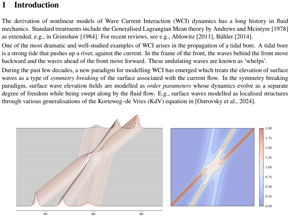
The central discovery is that the Burgers–swept KdV system, $$u_t+3uu_x=-v\partial_x($3v^{2}$+\gamma v_{xx}),\qquad v_t+6vv_x+\gamma v_{xxx}=-\partial_x(uv),$$ is best read through the Lie-transported momentum $m=u-\tfrac12 v^2$. If $m=0$ initially, the system reduces exactly to Gardner's equation for $v$, and the paper proves this reduction while giving closed-form compound soliton solutions and periodic travelling waves. Numerically, even with $m\neq0$ initial data, the system self-organizes into localized regions where $m\to0$, restoring Gardner dynamics and producing trains of compound solitons. In overtaking collisions, the simulations classify outcomes as refraction (the soliton slows, enters the bore, and leaves a wave train), reflection (the soliton exits the far side as a faster compound soliton carrying bore mass away), or fusion (two solitons merge near the bore front into one escaping soliton). The boundary between refraction and reflection is approximately $u_0\approx 5c$, i.e. $c_*\approx u_0/5$, in the small-amplitude regime.
Load-bearing premise
The collision classification and threshold $c_*\approx u_0/5$ are read from finite-time simulations that add viscosity $\eta=0.02$ to the Burgers equation to smooth the bore front, so the load-bearing premise is that this viscosity and the chosen resolution faithfully represent the dynamics of the inviscid system.
Editorial extensions
If this is right
- Localized emergence: if the $m\to0$ relaxation is generic, the asymptotic outcome of bore–soliton collisions is a train of compound Gardner solitons, opening the way to inverse-scattering methods for the final state.
- Predictive threshold: the reported relation $c_*\approx u_0/5$ means bore height and incident soliton speed alone decide, to leading order, whether an overtaking collision ends in absorption into the bore or escape ahead of it.
- Fusion changes soliton number: the bore can merge two solitons that would each be refracted into one reflected soliton, so the outgoing count is not fixed by the incoming count; identical, evenly spaced inputs can yield different numbers of escaping solitons as bore height changes.
- Closed-form benchmarks: the exact compound soliton and Jacobi-elliptic periodic solutions provide concrete initial data for testing simulations and reduced models of the interaction.
- Exact integrable subcase: whenever $m=0$ initially, Gardner-equation soliton dynamics persist exactly inside the coupled system; the paper's compound solitons are Gardner solitons modulated by an interaction factor $w(\xi)$.
Reading between the lines
- Threshold derivation: I would expect the $c_*\approx u_0/5$ line to follow from a momentum-flux balance at the bore front, so a matched-asymptotics or modulation-theory derivation should reproduce it independently of the numerical viscosity; if it cannot, the threshold is likely a numerical artifact.
- Generality to other wave equations: the same Doppler-shifted coupling applied to other integrable equations (modified KdV, nonlinear Schrödinger) should produce analogous refraction–reflection–fusion classifications, providing a sharp test of whether the threshold behaviour is universal.
- Integrability recurrence: the local return of $m$ to zero is reminiscent of recurrence of integrable behaviour in an infinite-dimensional system, making this model a concrete laboratory for the infinite-dimensional analogue of Fermi–Pasta–Ulam recurrence.
- Experimental signature: the theory predicts that in a controlled flume with a current of height $u_0$, an incident soliton with speed below about $0.2u_0$ (in the bore frame) is absorbed, while one above it escapes the bore as a faster soliton.
Signed reviews
Editorial analysis
A structured set of objections, weighed in public.
Referee Report
Summary. The paper studies the Burgers–swept KdV system (1), a coupled model of a Burgers-type current and a KdV-type wave field. It gives two variational derivations, shows that the momentum variable m = u - v^2/2 is Lie-transported, and observes that when m = 0 the system reduces to the integrable Gardner equation. Exact compound soliton solutions, solitary-wave relations, and periodic solutions are presented. The main numerical claims are that the system spontaneously creates regions with m → 0, that a Burgers bore interacting with compound solitons leads to refraction, reflection, or fusion depending on parameters, and that a threshold c* ≈ u0/5 separates refraction from reflection.
Significance. The variational derivation and the travelling-wave analysis are coherent and provide a useful geometric perspective on a wave–current interaction system. The explicit reduction to the Gardner equation for m = 0 is a clean structural observation, and the proposed classification of bore–soliton interactions is physically interesting if the numerical results are reliable. However, the numerical section as written is not reproducible: the simulated equation differs from system (1) by a factor of 3 in the Burgers nonlinearity, the viscosity parameter is stated inconsistently, and no resolution or convergence information is given. The exact soliton solution is also presented as a special m = 0 reduction rather than as a solution of the fully coupled system, which should be stated more carefully. With the numerical evidence repaired, the paper could make a solid contribution; in its current form the central numerical claims are not established.
major comments (3)
- [Section 3, first paragraph] The simulation equation is stated as u_t + u u_x = η u_xx − v ∂x(3v^2 + γ v_xx), but the system under study in (1) and in Eq. (30) is u_t + 3u u_x = −v ∂x(3v^2 + γ v_xx). The missing factor 3 changes the Burgers shock structure and the bore-front speed. Since the refraction/reflection threshold is defined in the bore's moving frame, the reported classification may be for a PDE different from system (1). The authors must state exactly which equation was integrated and provide the corresponding code or a detailed numerical specification.
- [Section 3 and Figure 7] The viscosity coefficient is set to η = 0.02 in the text of Section 3, while the caption of Figure 7 reports η = 0.01. In addition, no grid resolution, domain size, time step, or convergence tests are reported. The threshold c* ≈ u0/5 is read directly from these simulations, and without convergence and error quantification the numerical classification of refraction versus reflection is not supported as written.
- [Theorem 2.1 and Lemma 2.1] The 'exact compound soliton' of Theorem 2.1 is obtained by invoking Proposition 2.1, i.e., by assuming m = 0 initially, which reduces the system to the Gardner equation. The solution is therefore a Gardner soliton expressed in the (u,v) variables, not a solution of the fully coupled system with general m. This should be stated explicitly as a special reduced solution. In addition, Lemma 2.1 with u0 = 0 gives the condition (u−c)^2(u − v^2/2) = 0; the text selects u = v^2/2 without discussing the u = c branch, which is excluded only by the boundary condition u → 0 at infinity. This exclusion should be justified.
minor comments (3)
- [Remark 2.5 / Eq. (15)] Equation (15) appears to have a typo: integrating the travelling-wave equations gives (u(v) + 3v − c)v + γ v_xx = const, but the displayed equation omits the coefficient γ in front of v_xx.
- [Appendix A.1] The word 'auxialary' in the first sentence of Appendix A.1 is a typo for 'auxiliary'.
- [Figure 7] The caption defines x*(t) = argmax_x v(t), but the text does not specify how the refraction/reflection outcome is classified from the time series, nor how the threshold c* is extracted from the dashed lines. A precise classification criterion would help reproducibility.
Circularity Check
No significant circularity: the exact compound soliton is derived from the travelling-wave reduction, and the refraction/reflection/fusion claims rest on independent numerical observation.
full rationale
The paper's main derivations are self-contained and not circular. The exact compound soliton in Theorem 2.1 is not obtained by assuming the Gardner reduction; it follows from Lemma 2.1, whose travelling-wave relation (13) with soliton boundary conditions u0=0 forces u-v^2/2=0, hence m=0. The paper then correctly notes that the system reduces to Gardner under this derived constraint. The numerical claims in Section 3 (emergence of m→0, the refraction/reflection threshold c*≈u0/5, and fusion) are empirical simulation outcomes, not quantities fitted from data and then renamed as predictions. Self-citations to Holm et al. (2023) and Dombret et al. (2025) provide methodological background and prior proposal, but the variational derivation is re-derived in Section 2 and Appendix A with explicit variations, so no load-bearing argument reduces to a self-citation. One non-circular reproducibility concern should be flagged: Section 3 states the simulated viscous Burgers equation as 'u_t + u u_x = ηu_xx − v∂_x(3v^2+γv_xx)', whereas system (1) has 3u u_x in the Burgers term; additionally, the text gives η=0.02 while Figure 7's caption gives η=0.01. This is a correctness/reproducibility issue, not circularity, and does not change the circularity score.
Assumptions & free parameters
free parameters (2)
- η (viscosity) =
0.02 (Section 3), 0.01 (Figure 7)
- threshold coefficient in c* ≈ u0/5 =
5
assumptions (4)
- domain assumption The Dirac-Frenkel/Doppler-shifted variational coupling of Burgers and KdV Lagrangians is a valid model for wave-current interaction.
- standard math Known Gardner soliton and elliptic-function solutions.
- standard math Euler-Poincare reduction and the constrained variations δu = ∂t w - ad_u w.
- domain assumption Pseudo-spectral simulations with Dedalus accurately resolve the dynamics over the simulated time.
Cite this review
Pith. "Pith review of Compound Burgers-KdV Soliton Behaviour: Refraction, Reflection and Fusion." pith.science (2026). https://pith.science/paper/UZM3JB3S
@misc{pith2026250517026,
  author       = {Pith},
  title        = {Pith review of: Compound Burgers-KdV Soliton Behaviour: Refraction, Reflection and Fusion},
  year         = {2026},
  howpublished = {\url{https://pith.science/paper/UZM3JB3S}},
  note         = {Machine review of arXiv:2505.17026}
}
read the original abstract
We consider a coupled PDE system between the Burgers equation and the KdV equation to model the interactions between `bore'-like structures and wave-like solitons in shallow water. Two derivations of the resulting Burgers-swept KdV system are presented, based on Lie group symmetry and reduced variational principles. Exact compound soliton solutions are obtained, and numerical simulations show that the Burgers and KdV momenta tend toward a balance at which the coupled system reduces to the integrable Gardner equation. The numerical simulations also reveal rich nonlinear solution behaviours that include refraction, reflection, and soliton fusion, before the balance is finally achieved.
Figures


Figures from the paper (11 more)


Reference graph
Works this paper leans on
-
[1]
Mark J. Ablowitz. Nonlinear Dispersive Waves . Cambridge University Press, 9 2011. ISBN 9781107012547. doi:10.1017/CBO9780511998324
-
[2]
D. G. Andrews and M. E. Mcintyre. An exact theory of nonlinear waves on a lagrangian-mean flow. Journal of Fluid Mechanics, 89: 0 609--646, 12 1978. ISSN 0022-1120. doi:10.1017/S0022112078002773
-
[3]
Oliver B\" u hler. Waves and Mean Flows . Cambridge University Press, 3 2014. ISBN 9781107669666. doi:10.1017/CBO9781107478701
-
[4]
Keaton J. Burns , Geoffrey M. Vasil , Jeffrey S. Oishi , Daniel Lecoanet , and Benjamin P. Brown . Dedalus: A flexible framework for numerical simulations with spectral methods . Physical Review Research, 2 0 (2): 0 023068, April 2020. doi:10.1103/PhysRevResearch.2.023068
-
[5]
Albert Dombret, Darryl D. Holm, Ruiao Hu, Oliver D. Street, and Hanchun Wang. Collisions of Burgers Bores with Nonlinear Waves, pages 25--43. Springer International Publishing, 2025. doi:10.1007/978-3-031-70660-8_2
-
[6]
J. Frenkel. Wave mechanics: Advanced general theory . The Mathematical Gazette, 18: 0 208, 1934
work page 1934
-
[7]
Clifford S. Gardner, John M. Greene, Martin D. Kruskal, and Robert M. Miura. Method for Solving the Korteweg-deVries Equation . Phys. Rev. Lett., 19: 0 1095--1097, Nov 1967. doi:10.1103/PhysRevLett.19.1095
-
[8]
K. Gorshkov, I. Soustova, Alexey Ermoshkin, and N.V. Zaytseva. Evolution of the compound G ardner-equation soliton in the media with variable parameters. Radiophysics and Quantum Electronics, 55, 10 2012. doi:10.1007/s11141-012-9373-1
Show all 12 references
-
[9]
Wave action and wave-mean flow interaction, with application to stratified shear flows
R Grimshaw. Wave action and wave-mean flow interaction, with application to stratified shear flows. Annual Review of Fluid Mechanics, 16: 0 11--44, 1 1984. ISSN 0066-4189. doi:10.1146/annurev.fl.16.010184.000303
1984
-
[10]
Holm, Ruiao Hu, and Oliver D
Darryl D. Holm, Ruiao Hu, and Oliver D. Street. Lagrangian reduction and wave mean flow interaction. Physica D: Nonlinear Phenomena, 454: 0 133847, 2023. ISSN 0167-2789. doi:https://doi.org/10.1016/j.physd.2023.133847
2023
-
[11]
Localized wave structures: Solitons and beyond
L Ostrovsky, E Pelinovsky, V Shrira, and Y Stepanyants. Localized wave structures: Solitons and beyond. Chaos: An Interdisciplinary Journal of Nonlinear Science, 34 0 (6), 2024
2024
-
[12]
Particle description of the interaction between wave packets and point vortices
Nick Pizzo and Rick Salmon. Particle description of the interaction between wave packets and point vortices. Journal of Fluid Mechanics, 925: 0 A32, 2021. doi:10.1017/jfm.2021.661
2021 doi
Reviewed August 16, 2026 · model on record in the stance chip above.
Discussion (0). Continue with ORCID to comment.