Piecewise Linear Approximation in Learned Index Structures: Theoretical and Empirical Analysis

Guangyi Zhang; Jianwei Liao; Jiayong Qin; Jingshu Peng; Lei Chen; Qiyu Liu; Sha Hu; Xianyu Zhu; Yingxia Shao; Zhigang Cai

REVIEW 4 major objections 5 minor 61 references

Piecewise Linear Approximation in Learned Index Structures: Theoretical and Empirical Analysis

T0 review · 4 major / 5 minor · reviewed 2026-08-15 · deepseek-v4-flash

Challenge this review Re-run · record.json Download PDF Read on arXiv ↗ Review JSON

Pith's one-line read Segment coverage of learned indexes is Ω(κ ε²) on any key distribution.

desk verdict Useful benchmark, but the claimed Ω(κ ε²) lower bound is an artifact of a misdefined expectation in Eq. (2); with the correct tail-sum identity the proof gives only Ω(ε). read the letter →

arxiv 2506.20139 v1 pith:THM4IIEA submitted 2025-06-25 cs.DB cs.LG

Jiayong Qin , Xianyu Zhu , Qiyu Liu , Guangyi Zhang , Zhigang Cai , Jianwei Liao , Sha Hu , Jingshu Peng

show 2 more authors

Yingxia Shao Lei Chen

This is my paper · ORCID

classification cs.DBcs.LG

keywords piecewiselinearapproximationlearnedindexstructuressegmentcoveragelowerboundepsilon-PLAorderstatisticsPLABenchPGM-Index

verification ladder T0 review T1 audit T2 compute T3 formal

The pith

A machine-rendered reading of the paper's core claim, the machinery that carries it, and where it could break.

The reading

The paper targets a blind spot in learned index design: how many keys each linear segment covers when fitting an error-bounded piecewise linear model (ε-PLA). It claims a lower bound of Ω(κ ε²) on expected segment coverage that holds for both optimal and greedy fitting algorithms, assuming only that the sorted keys are drawn i.i.d. from an arbitrary bounded distribution, dropping the i.i.d.-gap assumption used in prior work. If right, this means index size shrinks quadratically with the error tolerance ε on any distribution, and greedy builders are asymptotically as good as optimal ones. The paper also benchmarks the algorithms inside FITing-Tree and PGM-Index, showing that greedy builders cut construction time by up to 3× at large ε while adding only modest space overhead.

What carries the argument

The machinery is order-statistics analysis of the residual δ_i = ℓ(K_(i)) − i between a fixed-slope line and the true index. Because K_(i) for i.i.d. keys follows a beta distribution in the uniform case and an asymptotically normal law in the general case, the residual has known variance; Chebyshev's inequality bounds each event |δ_j| ≤ ε, and a positive-correlation assumption turns the product of those probabilities into a sum that is Ω(ε²). The FRS algorithm—a proof device rather than a practical builder—carries the argument, and Theorem 5 uses a slope-range induction to show that SwingFilter and GreedyPLA cover every point FRS covers.

What would settle it

Compute, for large n and keys drawn from U(0,ρ), the exact joint probability Pr(∩_{j=1}^i {|δ_j| ≤ ε}) and compare it with the product ∏ Pr(|δ_j| ≤ ε); if for some i the joint probability falls below the product, inequality (5) and the Ω(ε²) lower bound do not follow from the given argument. A stronger empirical falsifier would be a distribution, such as a mixture with a near-point mass, where the measured segment coverage of OptimalPLA is o(ε²) for large n.

Watch

Extended reading notes

Core claim

The central claim is that the expected number of keys covered by a segment in any ε-PLA learned index is Ω(κ ε²), where κ is a data-dependent constant, for both optimal algorithms (ParaOptimal, SlideFilter, OptimalPLA) and greedy heuristics (SwingFilter, GreedyPLA). The proof works by constructing a Fixed Range Segmentation (FRS) algorithm that fixes the segment slope to (n+1)/ρ and then showing that any other ε-PLA fits at least as well; for uniform keys the coverage is Ω(ε²), and for arbitrary distributions it is Ω(√ρ(ε−γ)²/ξ) under mild conditions on the density and quantile approximation. Empirically, segment counts scale as 1/ε² on real and synthetic datasets, and the greedy algorithms produce at most a constant factor more segments than the optimum, with larger intra-segment residuals for the optimal fit explaining its slightly slower queries.

Load-bearing premise

The proof that segments cover Ω(κ ε²) keys relies on the events 'the j-th key lies within ε of the fixed line' being positively correlated, so that the probability all of the first i keys are covered is at least the product of the individual probabilities; the paper gives only an intuitive variance argument and defers a rigorous proof.

Editorial extensions

If this is right

Index size is quadratic in 1/ε: increasing the error bound from 32 to 128 shrinks the expected segment count by roughly 16×, independent of the data distribution up to the constant κ.
Greedy ε-PLA algorithms inherit the same Ω(κ ε²) coverage bound, so at large ε their segment counts converge to those of the optimal fitter.
Parallel construction raises the segment count by at most (threads − 1), making thread-level partitioning essentially free when the serial segment count m is much larger than the thread count.
The prior restriction ε ≫ σ/µ is unnecessary; the bound holds for small ε, the range most relevant for last-mile search in learned indexes.
A practical selection rule follows: use OptimalPLA for tight error bounds and switch to greedy builders when ε reaches about 2^5, saving up to half of construction time with comparable segment counts.

Reading between the lines

Editorial extensions of the paper, not claims the author makes directly.

If the positive-correlation assumption is repaired, the same Ω(κ ε²) argument likely extends to distributions with bounded support but non-smooth density at quantile points, since the proof uses only residual variance and mild regularity.
The fixed-slope analysis suggests a density-based view of the constant κ: datasets with steep density peaks should admit much larger κ and hence smaller indexes than the worst case, which could be tested by estimating κ from the empirical density.
The U-shaped query-time curves imply an optimal operating point in ε; a cost model that predicts the turning point from the residual distribution of the chosen PLA algorithm would turn the benchmark findings into a tuning rule.
A direct extension would apply the same residual analysis to recursive PGM layers, where each layer's input is itself a segment-count sequence rather than raw keys, to see whether the Ω(κ ε²) bound propagates layer by layer.

Share X Bluesky LinkedIn Reddit HN

Signed reviews

No signed human review yet.

Editorial analysis

A structured set of objections, weighed in public.

Desk editor's note, referee report, and a circularity audit.

Desk Editor's Note

read the letter

Short version: PLABench is a solid empirical contribution and worth having; the theoretical headline is not established. Eq. (2) defines expected segment coverage as E[I] = Σ i·Pr(E1∧...∧Ei), which is not the expectation of a run length. The correct identity is E[I] = Σ Pr(I ≥ i) = Σ Pr(E1∧...∧Ei), with no i factor. That extra factor is exactly what turns the final sum into Θ(ε²); without it the same Chebyshev-plus-product argument bottoms out at Θ(ε). So Theorem 3, and by extension Theorem 4, is not proven as written. This holds independently of the footnote-2 correlation issue; even if positive correlation were granted, the quadratic rate does not follow.

That said, the paper does several things well. Modeling keys directly as order statistics rather than i.i.d. gaps is the right instinct, and the authors correctly identify real limitations in the gap-based MET analysis for small ε and bounded integer keys. FRS is a clean proof device, and Theorem 5's argument that greedy algorithms dominate FRS is plausible. PLABench is genuinely useful: three PLA algorithms across two index structures, six datasets, parallel construction behavior, and Theorem 6's bound on segment increase from thread-level partitioning. The empirical observation that greedy PLA can beat optimal PLA on query latency despite generating more segments is a real and publishable finding.

Soft spots beyond Eq. (2): the positive-correlation assertion is explicitly deferred and is load-bearing; the arbitrary-distribution theorem inherits the same expectation flaw and also sweeps a bias term γ into the error; the claimed 'tightest' status rests on the invalid quadratic. If the authors fix the identity, the natural correct result for FRS is Ω(ε), which is weaker than the existing 2ε bound and not 'fundamentally improved.'

Who is this for? People building or tuning learned indexes will get value from the benchmark and the algorithm trade-offs. Theorists should not cite it for the lower bound until the proof is repaired. The paper deserves a serious referee, but the current version should not be accepted; it needs a corrected theoretical section before the claims become credible. If the benchmark is extracted or the theory is fixed, both parts can be published.

Referee Report

4 major / 5 minor

Summary. The paper studies error-bounded piecewise linear approximation (ε-PLA) for learned index structures. It claims a new lower bound Ω(κ·ε²) on the expected segment coverage for both optimal and greedy ε-PLA fitting algorithms under the assumption that keys are i.i.d. samples from an arbitrary distribution, relaxing earlier gap-based assumptions. The bound is stated in the abstract, formalized in Theorems 3 and 4, and extended to greedy algorithms via Theorem 5. The paper also introduces PLABench, a benchmark that integrates OptimalPLA, GreedyPLA, and SwingFilter into FITing-Tree and PGM-Index, empirically evaluating segment counts, construction time, index size, and query latency across six datasets.

Significance. If the theoretical bound were valid, the paper would make a meaningful contribution: it would provide the first coverage lower bound under i.i.d. keys rather than i.i.d. gaps, and it would explain observed quadratic behavior of segment counts. The empirical benchmark is also potentially useful, and the public release of PLABench is a strength, as are the reproducible comparisons across algorithms, structures, and datasets. However, the central proof of Ω(κ·ε²) is not valid as written. Definition 2 misstates the expectation of a run-length random variable, and the incorrect i-weighted sum is what produces the quadratic rate in the proof. Correcting this error leaves only Ω(ε) from the given argument, so the paper's main advertised result is unsupported. The benchmark findings about greedy-versus-optimal trade-offs remain interesting but do not compensate for the invalid theoretical core.

major comments (4)

[Section III-A, Eq. (2)] Eq. (2) defines C(ε) = E[I] = Σ_i i·Pr(E1∧...∧Ei). For a nonnegative integer random variable I, the correct tail-sum identity is E[I] = Σ_{i≥1} Pr(I ≥ i) = Σ_i Pr(E1∧...∧Ei). The weighted sum in Eq. (2) is E[I(I+1)/2], not E[I]. This is load-bearing: in Eqs. (4)–(7), the factor i is carried through the product bound and summed over i=1..ε, producing Θ(ε²). With the correct tail-sum formula, the same Chebyshev and product arguments give Σ_{i=1}^{ε} e^{-1/2} = Θ(ε), not Θ(ε²). Thus Theorem 3's proof does not establish the claimed Ω(ε²) coverage, and the abstract's central claim is unsupported by the written derivation.
[Section III-B, footnote 2 and Eq. (4)] The proof uses Pr(E1∧...∧Ei) ≥ ∏_{j=1}^i Pr(Ej) to obtain Eq. (4). This positive-correlation assertion is justified only by an intuitive variance-monotonicity remark in footnote 2, and the footnote explicitly defers a rigorous proof. The assertion is not evident: even though Var(δ_j) increases with j, the events E_j are dependent in a complex way through the order statistics, and variance growth alone does not imply positive association of the tail events. Since Eq. (4) and the subsequent product lower bound depend on this unproved inequality, the proof of Theorem 3 remains incomplete even if the expectation identity in Eq. (2) were corrected.
[Section III-C, Eqs. (10) and (11)] The variance of δ_i is given in Eq. (10) as i(n-i)/(ρ²·f(F^{-1}(i/n))²). Under the assumption f(F^{-1}(i/n)) ≥ 1/ξ, Chebyshev's inequality gives Pr(|δ_i - m_i| > ε) ≤ i(n-i)/(ρ² ε² f(...)²) ≤ i n ξ²/(ρ² ε²). The paper instead writes 1 - iξ²/(ρ ε²) in Eq. (11), which misses the factor n/ρ (or an equivalent normalization). Since ρ = Θ(n), n/ρ is not identically 1, and the missing factor affects the stated rate Ω(√ρ·(ε-γ)²/ξ). The proof of Theorem 4 therefore does not follow from the displayed variance calculation.
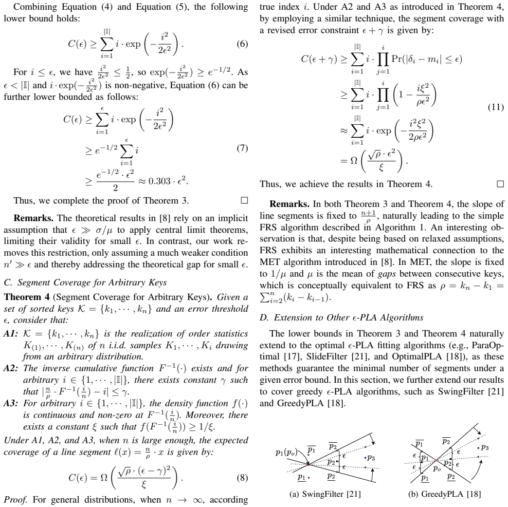
[Section III-D, Theorem 5] The induction in Theorem 5 compares a SwingFilter segment and an FRS segment that both start from the same first point. The argument shows that any point covered by FRS's initial segment is covered by SwingFilter's initial segment. However, when FRS later starts a new segment (because the fixed-slope segment violates the error bound), SwingFilter need not start a new segment at that same point; its current segment may continue, or it may have ended earlier. The proof does not establish a correspondence between subsequent FRS segments and SwingFilter segments, so the theorem's claim that SwingFilter and GreedyPLA always have larger segment coverage than FRS is not justified for segments after the first. Since Theorem 5 is the basis for extending the lower bound to greedy algorithms, this gap is load-bearing for that extension.

minor comments (5)

[Section III-A, Definition 2] The symbol I is used both for the random run length and for the set of possible values I={1,...,|I|}; clearer notation such as I and ℕ would avoid confusion. Also, the sentence claiming that the alternative Pr(E1∧...∧Ei∧Ei+1) is asymptotically equivalent is asserted without justification and is not obviously true under the correct tail-sum formulation.
[Section III-B, Theorem 3 proof] The proof refers to 'Theorem 2', but no Theorem 2 appears in the manuscript; this is presumably a numbering artifact or a missing reference and should be fixed.
[Section III-B, Eq. (5)] The approximation ∏(1 - j/((n+2)ε²)) ≈ exp(-Σ j/ε²) uses log(1-x)≈-x without stating conditions on the size of j/ε² relative to 1; for small ε the approximation and the subsequent e^{-1/2} bound need a uniform justification.
[Table VII] For SwingFilter on the books dataset, the reported 'Segments (Others)' for ε=2^3 is {791500,4463,27,2}, identical to the ε=2^2 row; this is likely a copy-and-paste error and should be checked.
[Section IV-B] The benchmark compiles with -O0 to ensure fairness; this is a reasonable choice but should be stated as limiting the performance conclusions to unoptimized builds, since real systems use -O2 or higher.

Circularity Check

1 steps flagged · score 8.0 of 10

The claimed Ω(κ ε²) coverage lower bound is produced by the i-weighted definition of C(ε) in Eq. (2), not by the order-statistics argument.

self definitional [Section III-A, Definition 2, Eq. (2); applied in Theorem 3 Eqs. (4)-(7) and Theorem 4 Eq. (11)]
"C(ε) = E[I] = Σ_{i∈I} i·Pr(E1∧E2···∧Ei), where Ei denotes the event of |ℓ(xi)−yi| ≤ ε, r.v. I represents the number of consecutive occurrences of Ei, and I={1,2,···,|I|} is the set of all possible values of i."

For a nonnegative integer r.v. I, the tail-sum identity is E[I]=Σ_{i≥1}Pr(I≥i)=Σ_i Pr(E1∧...∧Ei). The i-weighted right-hand side of Eq. (2) equals E[I(I+1)/2], not E[I]. The proof lower-bounds i·exp(−i²/2ε²) and sums to Θ(ε²) in Eq. (7); with the correct tail-sum formula, the same Chebyshev/product estimate gives only Θ(ε). Thus the central Ω(κε²) rate is inserted into the definition of coverage and recovered from it, rather than derived from the key distribution.

full rationale

The main circular step is Definition 2: C(ε) is defined via an i-weighted sum that is not the expectation of I. That i factor is load-bearing: dropping it (as the standard tail-sum identity requires) changes the theorem's conclusion from Ω(ε²) to Ω(ε) under the paper's own inequalities, so the claimed lower bound is a definitional artifact. Footnote 2 also explicitly defers the positive-correlation proof ('A more rigorous proof can be made by evaluating Pr(E_{j<i}|Ei), which is ignored here for brevity'), a correctness gap but not itself circularity. The benchmark does not fit parameters to produce the bound; the data-dependent constants ρ, ξ, γ, κ are assumptions about the input distribution, and the self-citations ([12]–[15], [34]) are not used to carry the proof. The empirical 'validation' in Figure 4 fits #Segments=a·ε^{-2}+b, which is descriptive rather than a prediction forced by the theory. Because the central theoretical claim reduces by construction to the definition of C(ε), the score is high despite the absence of self-citation circularity.

Assumptions & free parameters 3 free parameters · 4 assumptions · 0 invented entities

The central theoretical argument introduces no new entities. The FRS algorithm is a proof device, not a new physical or mathematical object. The free parameters rho, xi, gamma, kappa are data-dependent constants arising from the distributional assumptions, not fitted to data.

free parameters (3)

kappa (segment coverage constant) = unspecified; for uniform keys e^{-1/2}/2 is approximately 0.303, for arbitrary keys depends on rho and xi
The lower bound is stated as Omega(kappa * epsilon^2) without an explicit closed form for general distributions; kappa aggregates the effect of the key range rho and the density bound xi, which are data-dependent, not fitted to the experimental results.
rho (key range) = Theta(n), assumed
The paper assumes all keys lie in [0, rho] with rho = Theta(n). This is a modeling assumption that affects the slope n/rho of the FRS line and the variance of residuals.
xi (inverse density bound) = unspecified, assumed finite
Assumption A3 requires the key density f to be at least 1/xi at the quantiles of interest; xi controls the strength of the lower bound in Theorem 4.

assumptions (4)

domain assumption Keys are i.i.d. samples from an arbitrary continuous distribution (A1)
The proof models sorted keys as order statistics of n i.i.d. samples. This excludes duplicate keys and non-random key generation, and the bounded range assumption rho = Theta(n) is imposed additionally.
domain assumption Inverse CDF is approximately linear for the first segment: |(n/rho) * F^{-1}(i/n) - i| <= gamma (A2)
Used in Theorem 4 to bound the bias m_i of residuals; for strongly nonlinear CDFs (e.g., lognormal tails) this constant may be large and the bound weak.
domain assumption Density f is continuous and f(F^{-1}(i/n)) >= 1/xi (A3)
Ensures the asymptotic variance of order statistics is bounded from above; distributions with vanishing density in relevant regions are excluded.
ad hoc to paper Events E_j = {|ell(K_(j)) - j| <= epsilon} are positively correlated, so Pr(E_1 and ... and E_i) >= product of Pr(E_j)
This unproved assertion in footnote 2 of Section III-B is load-bearing: without it, the product lower bound in Equation (5) does not follow. The paper explicitly leaves the rigorous proof for future work.

how reviews work

0 comments

Cite this review

Pith. "Pith review of Piecewise Linear Approximation in Learned Index Structures: Theoretical and Empirical Analysis." pith.science (2026). https://pith.science/paper/THM4IIEA

@misc{pith2026250620139,
  author       = {Pith},
  title        = {Pith review of: Piecewise Linear Approximation in Learned Index Structures: Theoretical and Empirical Analysis},
  year         = {2026},
  howpublished = {\url{https://pith.science/paper/THM4IIEA}},
  note         = {Machine review of arXiv:2506.20139}
}

abstract

A growing trend in the database and system communities is to augment conventional index structures, such as B+-trees, with machine learning (ML) models. Among these, error-bounded Piecewise Linear Approximation ($\epsilon$-PLA) has emerged as a popular choice due to its simplicity and effectiveness. Despite its central role in many learned indexes, the design and analysis of $\epsilon$-PLA fitting algorithms remain underexplored. In this paper, we revisit $\epsilon$-PLA from both theoretical and empirical perspectives, with a focus on its application in learned index structures. We first establish a fundamentally improved lower bound of $\Omega(\kappa \cdot \epsilon^2)$ on the expected segment coverage for existing $\epsilon$-PLA fitting algorithms, where $\kappa$ is a data-dependent constant. We then present a comprehensive benchmark of state-of-the-art $\epsilon$-PLA algorithms when used in different learned data structures. Our results highlight key trade-offs among model accuracy, model size, and query performance, providing actionable guidelines for the principled design of future learned data structures.

Figures

Figures reproduced from arXiv: 2506.20139 by the authors.

**Figure 1.** Illustration of the ϵ-PLA model and learned index structure based on ϵ-PLA. ping from keys to their corresponding sorting indexes I = {1, · · · , n}, defined as f : K 7→ I. Intuitively, f can be regarded as the cumulative distribution function (CDF) of K, scaled by a factor of data size n. As illustrated in Figure 1a, existing fitting algorithms, such as SwingFilter [17] and GreedyPLA [18], can find an ϵ-PLA that a… view at source ↗

**Figure 2.** Illustration of segment coverage by constructing the [PITH_FULL_IMAGE:figures/full_fig_p004_2.png] view at source ↗

**Figure 3.** Illustration of two greedy ϵ-PLA fitting algorithms. The point in red (po) is the selected pivot point. As illustrated in [PITH_FULL_IMAGE:figures/full_fig_p005_3.png] view at source ↗

Figures from the paper (7 more)

**Figure 5.** Figure 5: Construction time w.r.t. ϵ ∈ {2 2 , 2 3 , · · · , 2 13} for different ϵ-PLA fitting algorithms. V. EXPERIMENTAL RESULTS In this section, we present the benchmark results addressing the research questions outlined earlier. Specifically, Section V-A reports the standal…

**Figure 6.** Figure 6: Increment of segment count w.r.t. the number of [PITH_FULL_IMAGE:figures/full_fig_p008_6.png]

**Figure 7.** Figure 7: Index size of FIT (FITing-Tree + ϵ-PLA) w.r.t. ϵ ∈ {2 2 , 2 3 , · · · , 2 13} for different ϵ-PLA algorithms. The fanout of the internal B+-tree is fixed to 16, so that each internal tree node occupies 256 bytes. that GreedyPLA and SwingFilter incur approximately 1.23×…

**Figure 10.** Figure 10: Query processing time of PGM (PGM-Index + [PITH_FULL_IMAGE:figures/full_fig_p010_10.png]

**Figure 11.** Figure 11: Index size time of PGM (PGM-Index + ϵ-PLA) w.r.t. ϵ ∈ {2 2 , 2 3 , · · · , 2 13} for different ϵ-PLA fitting algorithms. phenomenon because all the ϵ-PLA methods share almost the same height and the exact searching range (i.e., same ϵi and ϵℓ). To explain this, we ca…

**Figure 13.** Figure 13: Query time of PGM-Index with varying ϵℓ and ϵi based on different ϵ-PLA methods on fb, books, osm datasets ods compared to FITing-Tree. (e.g., when ϵ ∈ {2 4 , 2 5 , 2 6}, the building time of PGM-Index varies more significantly across different ϵ-PLA algorithms, where…

**Figure 14.** Figure 14: Query time of PGM-Index with varying ϵℓ and ϵi based on different ϵ-PLA methods on synthetic datasets GreedyPLA [18], and SwingRR [45] aim to minimize the number of segments while satisfying the error constraint. Despite the distinction between optimal and suboptimal …

Review history (2 revisions) →

Discussion (0). Continue with ORCID to comment.

Reference graph

Works this paper leans on

61 extracted references · 57 canonical work pages

[1]

The case for learned index structures,

T. Kraska, A. Beutel, E. H. Chi, J. Dean, and N. Polyzotis, “The case for learned index structures,” inProceedings of the 2018 international conference on management of data, 2018, pp. 489–504

work page 2018
[2]

A model for learned bloom filters and optimizing by sandwiching,

M. Mitzenmacher, “A model for learned bloom filters and optimizing by sandwiching,”Advances in Neural Information Processing Systems, vol. 31, 2018

work page 2018
[3]

Effectively learning spatial indices,

J. Qi, G. Liu, C. S. Jensen, and L. Kulik, “Effectively learning spatial indices,”Proceedings of the VLDB Endowment, vol. 13, no. 12, pp. 2341–2354, 2020

work page 2020
[4]

Benchmarking learned indexes,

R. Marcus, A. Kipf, A. van Renen, M. Stoian, S. Misra, A. Kemper, T. Neumann, and T. Kraska, “Benchmarking learned indexes,”Proceed- ings of the VLDB Endowment, vol. 14, no. 1, pp. 1–13, 2020

work page 2020
[5]

Are up- datable learned indexes ready?

C. Wongkham, B. Lu, C. Liu, Z. Zhong, E. Lo, and T. Wang, “Are up- datable learned indexes ready?”Proceedings of the VLDB Endowment, vol. 15, no. 11, pp. 3004–3017, 2022

work page 2022
[6]

The pgm-index: a fully-dynamic com- pressed learned index with provable worst-case bounds,

P. Ferragina and G. Vinciguerra, “The pgm-index: a fully-dynamic com- pressed learned index with provable worst-case bounds,”Proceedings of the VLDB Endowment, vol. 13, no. 8, pp. 1162–1175, 2020

work page 2020
[7]

Deep learning,

Y . LeCun, Y . Bengio, and G. Hinton, “Deep learning,”nature, vol. 521, no. 7553, pp. 436–444, 2015

2015
[8]

Why are learned indexes so effective?

P. Ferragina, F. Lillo, and G. Vinciguerra, “Why are learned indexes so effective?” inInternational Conference on Machine Learning. PMLR, 2020, pp. 3123–3132

work page 2020

Show all 61 references

[9]

Fiting-tree: A data-aware index structure,

A. Galakatos, M. Markovitch, C. Binnig, R. Fonseca, and T. Kraska, “Fiting-tree: A data-aware index structure,” inProceedings of the 2019 international conference on management of data, 2019, pp. 1189–1206

2019
[10]

Learned index with dynamicϵ,

D. Chen, W. Li, Y . Li, B. Ding, K. Zeng, D. Lian, and J. Zhou, “Learned index with dynamicϵ,” inICLR. OpenReview.net, 2023

2023
[11]

From{WiscKey}to bourbon: A learned index for{Log-Structured}merge trees,

Y . Dai, Y . Xu, A. Ganesan, R. Alagappan, B. Kroth, A. Arpaci-Dusseau, and R. Arpaci-Dusseau, “From{WiscKey}to bourbon: A learned index for{Log-Structured}merge trees,” in14th USENIX Symposium on Operating Systems Design and Implementation (OSDI 20), 2020, pp. 155–171

2020
[12]

Lhist: towards learning multi-dimensional histogram for massive spatial data,

Q. Liu, Y . Shen, and L. Chen, “Lhist: towards learning multi-dimensional histogram for massive spatial data,” in2021 IEEE 37th International Conference on Data Engineering (ICDE). IEEE, 2021, pp. 1188–1199

2021
[13]

HAP: an efficient hamming space index based on augmented pigeonhole principle,

——, “HAP: an efficient hamming space index based on augmented pigeonhole principle,” inProceedings of the 2022 International Confer- ence on Management of Data, 2022, pp. 917–930

2022
[14]

Bittuner: A toolbox for automatically configuring learned data compressors,

Q. Liu, Y . Luo, M. Cui, S. Han, J. Peng, J. Li, and L. Chen, “Bittuner: A toolbox for automatically configuring learned data compressors,” in 2025 IEEE 41st International Conference on Data Engineering (ICDE). IEEE Computer Society, 2025, pp. 4548–4551

2025
[15]

Learned data compression: Challenges and opportunities for the future,

Q. Liu, S. Han, J. Liao, J. Li, J. Peng, J. Du, and L. Chen, “Learned data compression: Challenges and opportunities for the future,”arXiv preprint arXiv:2412.10770, 2024

2024 arXiv
[16]

Organization and maintenance of large ordered indices,

R. Bayer and E. McCreight, “Organization and maintenance of large ordered indices,” inProceedings of the 1970 ACM SIGFIDET (Now SIGMOD) Workshop on Data Description, Access and Control, 1970, pp. 107–141

1970
[17]

An on-line algorithm for fitting straight lines between data ranges,

J. O’Rourke, “An on-line algorithm for fitting straight lines between data ranges,”Commun. ACM, vol. 24, no. 9, pp. 574–578, 1981

1981
[18]

Maximum error- bounded piecewise linear representation for online stream approxima- tion,

Q. Xie, C. Pang, X. Zhou, X. Zhang, and K. Deng, “Maximum error- bounded piecewise linear representation for online stream approxima- tion,”VLDB J., vol. 23, no. 6, pp. 915–937, 2014

2014
[19]

Piece-wise linear approximations,

S. H. Cameron, “Piece-wise linear approximations,”Technical note CSTN-106, Computer Sciences Division, IIT Research Institute, Chicago, IL, 1966

1966
[20]

Time series compression survey,

G. Chiarot and C. Silvestri, “Time series compression survey,”ACM Computing Surveys, vol. 55, no. 10, pp. 1–32, 2023

2023
[21]

Online piece-wise linear approximation of numerical streams with precision guarantees,

H. Elmeleegy, A. K. Elmagarmid, E. Cecchet, W. G. Aref, and W. Zwaenepoel, “Online piece-wise linear approximation of numerical streams with precision guarantees,”Proceedings of the VLDB Endow- ment, vol. 2, no. 1, pp. 145–156, 2009

2009
[22]

A learned approach to design compressed rank/select data structures,

A. Boffa, P. Ferragina, and G. Vinciguerra, “A learned approach to design compressed rank/select data structures,”ACM Transactions on Algorithms (TALG), vol. 18, no. 3, pp. 1–28, 2022

2022
[23]

Techniques for inverted index compres- sion,

G. E. Pibiri and R. Venturini, “Techniques for inverted index compres- sion,”ACM Computing Surveys (CSUR), vol. 53, no. 6, pp. 1–36, 2020

2020
[24]

Handbook of stochastic methods for physics, chemistry and the natural sciences,

C. W. Gardiner, “Handbook of stochastic methods for physics, chemistry and the natural sciences,”Springer series in synergetics, 1985

1985
[25]

Redner,A guide to first-passage processes

S. Redner,A guide to first-passage processes. Cambridge university press, 2001

2001
[26]

J. E. Gentle,Computational statistics. Springer, 2009, vol. 308

2009
[27]

Entropic central limit theorem for order statistics,

M. Cardone, A. Dytso, and C. Rush, “Entropic central limit theorem for order statistics,”IEEE Transactions on Information Theory, vol. 69, no. 4, pp. 2193–2205, 2022

2022
[28]

Fast parallel operations on search trees,

Y . Akhremtsev and P. Sanders, “Fast parallel operations on search trees,” in2016 IEEE 23rd International Conference on High Performance Computing (HiPC). IEEE, 2016, pp. 291–300

2016
[29]

PGM-Index,

“PGM-Index,” https://github.com/gvinciguerra/PGM-index, accessed: 2025-06-10

2025
[30]

STX B+ Tree C++ template classes,

“STX B+ Tree C++ template classes,” https://panthema.net/2007/ stx-btree/, accessed: 2025-06-10

2007
[31]

Benchmarking learned indexes,

R. Marcus, A. Kipf, A. van Renen, M. Stoian, S. Misra, A. Kemper, T. Neumann, and T. Kraska, “Benchmarking learned indexes,”Proc. VLDB Endow., vol. 14, no. 1, p. 1–13, Sep. 2020

2020
[32]

Efficiently searching in-memory sorted arrays: Revenge of the interpolation search?

P. Van Sandt, Y . Chronis, and J. M. Patel, “Efficiently searching in-memory sorted arrays: Revenge of the interpolation search?” in Proceedings of the 2019 International Conference on Management of Data, ser. SIGMOD ’19, New York, NY , USA, 2019, p. 36–53. [Online]. Available...

2019
[33]

Openstreetmap,

openstreetmap, “Openstreetmap,” [n.d.]. [Online]. Available: https: //www.openstreetmap.org/
[34]

Why are learned indexes so effective but sometimes ineffective?

Q. Liu, S. Han, Y . Qi, J. Peng, J. Li, L. Lin, and L. Chen, “Why are learned indexes so effective but sometimes ineffective?”arXiv preprint arXiv:2410.00846, 2024

2024 arXiv
[35]

Adaptive sequential segmentation of piecewise stationary time series,

U. Appel and A. V . Brandt, “Adaptive sequential segmentation of piecewise stationary time series,”Information sciences, vol. 29, no. 1, pp. 27–56, 1983

1983
[36]

On the approximation of curves by line segments using dynamic programming,

R. Bellman, “On the approximation of curves by line segments using dynamic programming,”Communications of the ACM, vol. 4, no. 6, p. 284, 1961

1961
[37]

Computing unrestricted synopses under maximum error bound,

C. Pang, Q. Zhang, X. Zhou, D. Hansen, S. Wang, and A. Maeder, “Computing unrestricted synopses under maximum error bound,”Algo- rithmica, vol. 65, pp. 1–42, 2013

2013
[38]

Wavelet synopses for general error metrics,

M. Garofalakis and A. Kumar, “Wavelet synopses for general error metrics,”ACM Transactions on Database Systems (TODS), vol. 30, no. 4, pp. 888–928, 2005

2005
[39]

An online pla algorithm with maximum error bound for generating optimal mixed- segments,

H. Zhao, T. Li, G. Chen, Z. Dong, M. Bo, and C. Pang, “An online pla algorithm with maximum error bound for generating optimal mixed- segments,”International Journal of Machine Learning and Cybernetics, vol. 11, pp. 1483–1499, 2020

2020
[40]

Efficient algorithms for sequence segmen- tation,

E. Terzi and P. Tsaparas, “Efficient algorithms for sequence segmen- tation,” inProceedings of the 2006 SIAM International Conference on Data Mining. SIAM, 2006, pp. 316–327

2006
[41]

Optimal segmented linear re- gression for financial time series segmentation,

C.-J. Wu, W.-S. Zeng, and J.-M. Ho, “Optimal segmented linear re- gression for financial time series segmentation,” in2021 International Conference on Data Mining Workshops (ICDMW), 2021, pp. 623–630

2021
[42]

Segmenting time series: A survey and novel approach,

E. Keogh, S. Chu, D. Hart, and M. Pazzani, “Segmenting time series: A survey and novel approach,”Data Mining in Time Series Databases, vol. 57, 03 2003

2003
[43]

Novel online methods for time series segmentation,

X. Liu, Z. Lin, and H. Wang, “Novel online methods for time series segmentation,”IEEE Transactions on Knowledge and Data Engineering, vol. 20, no. 12, pp. 1616–1626, 2008

2008
[44]

A novel segmentation and representation approach for streaming time series,

Y . Hu, P. Guan, P. Zhan, Y . Ding, and X. Li, “A novel segmentation and representation approach for streaming time series,”IEEE Access, vol. 7, pp. 184 423–184 437, 2019

2019
[45]

A novel bounded-error piece- wise linear approximation algorithm for streaming sensor data in edge computing,

J.-W. Lin, S.-w. Liao, and F.-Y . Leu, “A novel bounded-error piece- wise linear approximation algorithm for streaming sensor data in edge computing,” inAdvances in Intelligent Networking and Collaborative Systems, L. Barolli, H. Nishino, and H. Miwa, Eds. Cham: Springer Inter...

2020
[46]

Ubiquitous b-tree,

D. Comer, “Ubiquitous b-tree,”ACM Comput. Surv., vol. 11, no. 2, p. 121–137, Jun. 1979

1979
[47]

Fast: fast architecture sensitive tree search on modern cpus and gpus,

C. Kim, J. Chhugani, N. Satish, E. Sedlar, A. D. Nguyen, T. Kaldewey, V . W. Lee, S. A. Brandt, and P. Dubey, “Fast: fast architecture sensitive tree search on modern cpus and gpus,” inProceedings of the 2010 ACM SIGMOD International Conference on Management of Data, ser. SIGM...

2010
[48]

Wormhole: A fast ordered index for in- memory data management,

X. Wu, F. Ni, and S. Jiang, “Wormhole: A fast ordered index for in- memory data management,” ser. EuroSys ’19. New York, NY , USA: Association for Computing Machinery, 2019

2019
[49]

Alex: an updatable adaptive learned index,

J. Ding, U. F. Minhas, J. Yu, C. Wang, J. Do, Y . Li, H. Zhang, B. Chandramouli, J. Gehrke, D. Kossmannet al., “Alex: an updatable adaptive learned index,” inProceedings of the 2020 ACM SIGMOD International Conference on Management of Data, 2020, pp. 969–984

2020
[50]

Xindex: a scalable learned index for multicore data storage,

C. Tang, Y . Wang, Z. Dong, G. Hu, Z. Wang, M. Wang, and H. Chen, “Xindex: a scalable learned index for multicore data storage,” in Proceedings of the 25th ACM SIGPLAN Symposium on Principles and Practice of Parallel Programming, ser. PPoPP ’20. New York, NY , USA: Association...

2020
[51]

Finedex: a fine-grained learned index scheme for scalable and concurrent memory systems,

P. Li, Y . Hua, J. Jia, and P. Zuo, “Finedex: a fine-grained learned index scheme for scalable and concurrent memory systems,”Proc. VLDB Endow., vol. 15, no. 2, p. 321–334, Oct. 2021

2021
[52]

G-learned index: Enabling efficient learned index on gpu,

J. Liu, F. Zhang, L. Lu, C. Qi, X. Guo, D. Deng, G. Li, H. Zhang, J. Zhai, H. Zhang, Y . Chen, A. Pan, and X. Du, “G-learned index: Enabling efficient learned index on gpu,”IEEE Transactions on Parallel and Distributed Systems, vol. 35, no. 6, pp. 950–967, 2024

2024
[53]

Carmi: a cache-aware learned index with a cost- based construction algorithm,

J. Zhang and Y . Gao, “Carmi: a cache-aware learned index with a cost- based construction algorithm,”Proc. VLDB Endow., vol. 15, no. 11, p. 2679–2691, Jul. 2022

2022
[54]

Making in-memory learned indexes efficient on disk,

J. Zhang, K. Su, and H. Zhang, “Making in-memory learned indexes efficient on disk,”Proc. ACM Manag. Data, vol. 2, no. 3, May 2024

2024
[55]

Ferragina, Paoloand Vinciguerra,Learned Data Structures

G. Ferragina, Paoloand Vinciguerra,Learned Data Structures. Cham: Springer International Publishing, 2020, pp. 5–41

2020
[56]

Semantic hashing,

R. Salakhutdinov and G. Hinton, “Semantic hashing,”International Journal of Approximate Reasoning, vol. 50, no. 7, pp. 969–978, 2009, special Section on Graphical Models and Information Retrieval

2009
[57]

Spectral hashing,

Y . Weiss, A. Torralba, and R. Fergus, “Spectral hashing,” inProceedings of the 22nd International Conference on Neural Information Processing Systems, ser. NIPS’08. Red Hook, NY , USA: Curran Associates Inc., 2008, p. 1753–1760

2008
[58]

A model for learned bloom filters, and optimizing by sandwiching,

M. Mitzenmacher, “A model for learned bloom filters, and optimizing by sandwiching,” inProceedings of the 32nd International Conference on Neural Information Processing Systems, ser. NIPS’18. Red Hook, NY , USA: Curran Associates Inc., 2018, p. 462–471

2018
[59]

Meta-learning neural bloom filters,

J. Rae, S. Bartunov, and T. Lillicrap, “Meta-learning neural bloom filters,” inInternational Conference on Machine Learning. PMLR, 2019, pp. 5271–5280

2019
[60]

Stable learned bloom filters for data streams,

Q. Liu, L. Zheng, Y . Shen, and L. Chen, “Stable learned bloom filters for data streams,”Proceedings of the VLDB Endowment, vol. 13, no. 12, pp. 2355–2367, 2020

2020
[61]

Learning-based fre- quency estimation algorithms

C.-Y . Hsu, P. Indyk, D. Katabi, and A. Vakilian, “Learning-based fre- quency estimation algorithms.” inInternational Conference on Learning Representations, 2019

2019

Pith tools

Reviewed August 15, 2026 · model on record in the stance chip above.

[1] [1]

The case for learned index structures,

T. Kraska, A. Beutel, E. H. Chi, J. Dean, and N. Polyzotis, “The case for learned index structures,” inProceedings of the 2018 international conference on management of data, 2018, pp. 489–504

work page 2018

[2] [2]

A model for learned bloom filters and optimizing by sandwiching,

M. Mitzenmacher, “A model for learned bloom filters and optimizing by sandwiching,”Advances in Neural Information Processing Systems, vol. 31, 2018

work page 2018

[3] [3]

Effectively learning spatial indices,

J. Qi, G. Liu, C. S. Jensen, and L. Kulik, “Effectively learning spatial indices,”Proceedings of the VLDB Endowment, vol. 13, no. 12, pp. 2341–2354, 2020

work page 2020

[4] [4]

Benchmarking learned indexes,

R. Marcus, A. Kipf, A. van Renen, M. Stoian, S. Misra, A. Kemper, T. Neumann, and T. Kraska, “Benchmarking learned indexes,”Proceed- ings of the VLDB Endowment, vol. 14, no. 1, pp. 1–13, 2020

work page 2020

[5] [5]

Are up- datable learned indexes ready?

C. Wongkham, B. Lu, C. Liu, Z. Zhong, E. Lo, and T. Wang, “Are up- datable learned indexes ready?”Proceedings of the VLDB Endowment, vol. 15, no. 11, pp. 3004–3017, 2022

work page 2022

[6] [6]

The pgm-index: a fully-dynamic com- pressed learned index with provable worst-case bounds,

P. Ferragina and G. Vinciguerra, “The pgm-index: a fully-dynamic com- pressed learned index with provable worst-case bounds,”Proceedings of the VLDB Endowment, vol. 13, no. 8, pp. 1162–1175, 2020

work page 2020

[7] [7]

Deep learning,

Y . LeCun, Y . Bengio, and G. Hinton, “Deep learning,”nature, vol. 521, no. 7553, pp. 436–444, 2015

2015

[8] [8]

Why are learned indexes so effective?

P. Ferragina, F. Lillo, and G. Vinciguerra, “Why are learned indexes so effective?” inInternational Conference on Machine Learning. PMLR, 2020, pp. 3123–3132

work page 2020