REVIEW 3 major objections 4 minor 5 cited by
Ray-tracing Fast Radio Bursts Through IllustrisTNG: Cosmological Dispersion Measures from Redshift 0 to 5.5
T0 review · 3 major / 4 minor · reviewed 2026-08-06 · deepseek-v4-flash
Pith's one-line read Continuous ray tracing through the Voronoi mesh of a cosmological simulation corrects fast radio burst dispersion measures that sparse-snapshot methods had distorted by over 50%.
desk verdict Genuine methodological advance in FRB ray tracing through TNG; the central claim is plausible but the untested temporal snapshot discretization should be settled before p(DM|z) is taken as ground truth. read the letter →
The pith
A machine-rendered reading of the paper's core claim, the machinery that carries it, and where it could break.
The reading
What carries the argument
The load-bearing mechanism is the tilted continuous ray through the periodic simulation volume, with direction vector $\mathbf{n}=(1,5,25)$ and its twelve signed permutations; the coprime integer components make the repetition length $L_r \approx 27L$ for a box of side $L=205\,h^{-1}\,\mathrm{Mpc}$, so the ray does not re-cross the same structures. Along each ray, a recursive plane-crossing algorithm reconstructs every Voronoi cell the ray enters, so the electron density integral is evaluated on the true moving mesh rather than a Cartesian grid, avoiding what the paper estimates as a 1-10% gridding bias at $10^4$ bins. This machine, cross-checked against a stacked method that randomly rotates and shifts boxes, is what lets the paper claim the continuous catalog correctly captures cosmic variance.
What would settle it
Recompute the continuous catalog with additional snapshots inserted between the existing outputs (for example at every 0.1 in redshift, or at least at $z=1.5, 2.5, 3.5, 4.5$) and compare the standard deviation, skewness, and kurtosis of $p(\mathrm{DM}|z)$; if any moment shifts by more than a few percent, the piecewise-constant snapshot sampling is biasing the results the paper presents as corrected.
Extended reading notes
Core claim
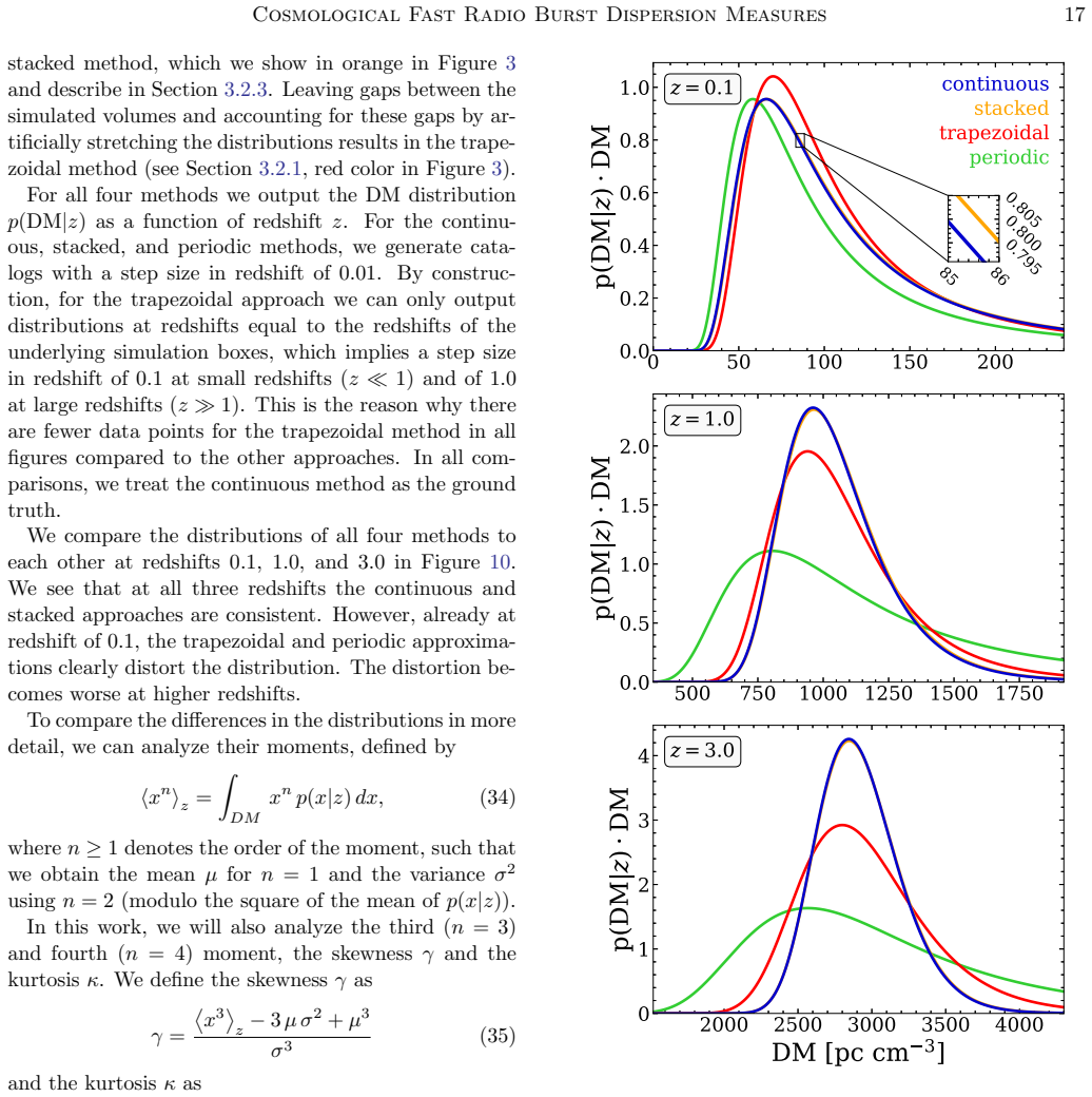
The central claim is that the way gaps between simulation snapshots are handled controls the higher moments of $p(\mathrm{DM}|z)$, not just its mean. The trapezoidal and periodic methods stretch each snapshot's DM distribution so the mean is correct, but this inflates the standard deviation by more than 50% (trapezoidal) and over 200% (periodic) relative to the continuous ground truth, with skewness and kurtosis distorted by tens to hundreds of percent. The continuous method sends tilted rays through the periodic box with direction $\mathbf{n}=(1,5,25)$, making the repetition length far longer than the box, and reconstructs all traversed Voronoi cell segments so dense small-scale structure is preserved. It yields over 20 public catalogs, including a full-sky DM map from a Milky Way-like environment, and a functional form $p_{\mathrm{np,31}}$ with $\alpha=1$, $\beta=3.3$ that fits $p(\mathrm{DM}|z)$ from $z=0$ to $5.5$, with simulated DMs consistent with the DSA-110, ASKAP, and CHIME samples.
Load-bearing premise
The continuous method still represents the electron density as constant within each of thirteen snapshot intervals, using one snapshot for the entire comoving segment to the next; if the real electron field changes significantly within a segment, especially where snapshots are one redshift unit apart, the corrected moments inherit that untested bias.
Editorial extensions
If this is right
- Previously published TNG-based dispersion measure distributions from trapezoidal or periodic stacking overstate the width and tails of $p(\mathrm{DM}|z)$, so conclusions about cosmic baryons drawn from those distributions should be rechecked.
- The $p_{\mathrm{np,31}}$ fit with $\alpha=1$ and $\beta=3.3$ gives a two-parameter, redshift-evolving prior for FRB dispersion measures that can replace the log-normal model in future analyses.
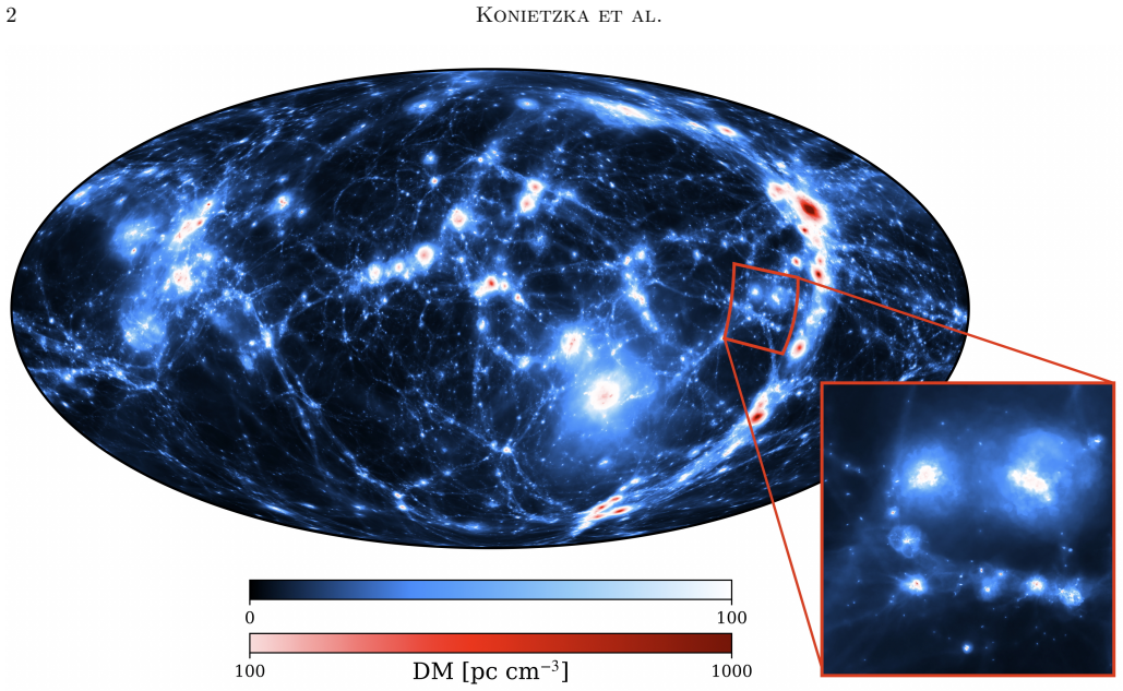
- The full-sky DM maps allow mock FRB samples with realistic sky positions, enabling forecasts for stacking analyses and for the FRB DM-galaxy angular cross-power spectrum.
- DM catalogs from boxes smaller than $35\,h^{-1}\,\mathrm{Mpc}$ or with baryonic resolution poorer than $5\times10^8\,h^{-1}\,M_\odot$ deviate from converged results by more than 8%, setting a quantitative floor for simulation choices in FRB work.
Reading between the lines
- The paper does not test whether its own piecewise-constant snapshot sampling biases moments, especially above $z=1$ where snapshots are one redshift unit apart; a rerun with intermediate snapshots would settle this.
- The same Voronoi segment-reconstruction ray tracing could be applied to other moving-mesh simulations and to other line-of-sight integrals such as the kinetic Sunyaev-Zeldovich signal, where snapshot sampling could produce analogous moment bias.
- The fitted exponents $\alpha\approx1$ and $\beta\approx3.3$ are interpreted by the paper as encoding halo electron content and the shape of dense cosmic web structures; connecting them to feedback parameters in simulation suites that vary feedback would be a natural next step.
- The paper's box size and resolution thresholds suggest some published small-box or low-resolution FRB forecasts, including those using lighter simulation suites, may carry an unaccounted >8% distortion of the DM distribution.
Editorial analysis
A structured set of objections, weighed in public.
Referee Report
Summary. The paper develops a Voronoi-segment ray tracer for computing FRB dispersion measures through IllustrisTNG, compares four integration schemes (trapezoidal, periodic, stacked, continuous), and releases over 20 DM catalogs. It argues that trapezoidal and periodic methods misestimate the variance and higher moments of p(DM|z), proposes a modified-normal power-law fit pnp,31 for p(DM|z), presents full-sky maps from Milky Way-like environments, checks resolution and box-size effects, and compares with FRB observations from DSA-110, ASKAP, and CHIME.
Significance. The methodological comparison is instructive: the toy Gaussian convolution example in Sec. 3.2.1 is a clean demonstration of why stretching snapshot distributions inflates variance, and the public catalogs and full-sky maps are useful community assets. If the central claim holds, the paper corrects a systematic error in previous TNG-based FRB work and provides a practical fitting function. The claim is currently conditional, however, because the 'ground truth' continuous method shares the same sparse snapshot sampling that it criticizes in other methods, and the fit and observational comparisons have not been quantitatively validated.
major comments (3)
- [Sec. 3.2.4, Eq. (27); Sec. 4.1, Fig. 11] The continuous method still represents the electron density with 13 discrete snapshots, each used over the full comoving segment between neighboring snapshot midpoints; at z > 1 these segments are Delta z = 1 wide. The paper criticizes sparse snapshot sampling in previous work, but it never tests whether this piecewise-constant time discretization biases the standard deviation, skewness, or kurtosis of p(DM|z). The agreement between the continuous and stacked methods in Sec. 4.1 does not settle this, because both methods use the same 13 snapshots and therefore share any common snapshot-discretization bias. A convergence test with higher-cadence outputs or interpolated density fields is needed, demonstrating stability of the moments and of the pnp,31 parameters. Without it, the 'ground truth' status of the continuous catalog, and hence the >50% misestimation claim and the observational comparison, are not fully established.
- [Sec. 4.2, Fig. 14] The shape parameters alpha ~ 1 and beta ~ 3.3 are optimized on the same six redshift slices (0.1, 0.5, 1.0, 1.5, 3.0, 5.0) that are then scored with the KS statistic in Fig. 14. This is an in-sample model comparison: the figure shows that pnp,31 fits the calibration data, not that it generalizes. Please provide a held-out validation (e.g., cross-validation across redshift slices) and report the uncertainty on alpha and beta, including sensitivity to binning and slice weighting. The statement that pnp,31 has 'only two free parameters' is also misleading because alpha and beta are fitted to the same data that are used for model selection.
- [Sec. 4.3, Fig. 15] The claimed consistency with DSA-110, ASKAP, and CHIME is supported only by visual inspection of the right panel of Fig. 15. No quantitative goodness-of-fit is presented, and the comparison depends on the host DM distribution (log-normal with mu_host = 4.9, sigma_host = 0.56) taken from Connor et al. (2025), which shares authorship with this paper. Please add a statistical test that accounts for the survey selection function and redshift uncertainties, and test the sensitivity of the conclusion to the host DM model and to the Milky Way DM subtraction.
minor comments (4)
- [Sec. 3.2.4, Eq. (27)] Equation (27) as typeset does not appear to produce the midpoint segmentation described in the text; for the listed snapshot redshifts it would give zero-length segments for alternating snapshots. Please correct the equation or clarify whether L_i is a segment length or a cumulative path length.
- [Sec. 3.2.3] The stacked method is described as 'yellow color in Figure 3', but Figure 3 and the rest of the text use orange; please make the color naming consistent.
- [Sec. 4.2] The KS statistics in Figure 14 should state the number of samples per redshift slice and whether the per-slice parameters mu and sigma are re-fitted independently for each model; this is needed to interpret the comparison.
- [Sec. 3.2] There are typographical issues such as 'commoving' instead of 'comoving' in Section 3.2 and the unusual spacing in 'F ast' in the Introduction; please proofread the manuscript.
Circularity Check
The analytic mean check is a fitted-input closure test, while the central method-comparison claim rests on inter-method comparisons and a toy model.
-
fitted input called prediction
[Section 4.3, Figure 15 (left panel), using feb(z) fit of Figure 17 and Eq. (9) from Section 2.2]
"To this end, we must first determine the behavior of the fraction of the dispersive electron density relative to the total baryon density feb(z) in IllustrisTNG. ... we model feb(z) ≈ feb,0 + feb,1 z. ... Using the linear fit to the evolution of the fraction of the dispersive electron density compared to the total baryon density, feb(z), we can calculate the integral defined in equation (9) and compare it with the evolution of p(DM|z) derived from the continuous catalog. ... We see that the analytical description perfectly describes the mean of the ray-tracing approach."
feb(z) is not an independent analytic input; it is measured from the same IllustrisTNG simulation whose ray-traced DM is being checked (Figure 17). Equation (9), via Eq. (7) where feb is defined by ⟨ne⟩ = feb ρb/mp, is just the redshift integral of the simulation's own mean electron density. The 'analytical description' matching the continuous catalog's mean is therefore a closure test of how well the ray ensemble reproduces the volume-averaged density, not an independent confirmation. The agreement is nearly forced by construction, so presenting it as an analytical confirmation overstates its evidential weight. This step is not load-bearing for the paper's central higher-moment claim, which is supported by inter-method comparisons and the toy-model argument in Section 3.2.1.
full rationale
The paper's main quantitative claim—that trapezoidal and periodic ray-tracing distort the standard deviation, skewness, and kurtosis by over 50%—is not circular: it is a direct comparison of four integration schemes on the same TNG density fields, supported by an analytic toy example (Eqs. 20-22) that shows why gap-stretching biases the variance. The continuous/stacked agreement is cross-method consistency, and the full-sky/continuous/random comparisons are internal validations rather than reductions to inputs. The one genuinely circular-looking step is the 'analytic confirmation' of the mean DM-redshift relation (Section 4.3, Figure 15): feb(z) is fitted from the same simulation, and Eq. (9) simply integrates that measured mean electron density, so the near-perfect agreement is a closure test, not an independent analytical prediction. This is fitted input called prediction in a mild form, but it is not central to the main claim. The host-DM log-normal parameters are taken from Connor et al. (2025), a paper with overlapping authorship, but they are an observational fit applied as an external input rather than derived here; this is normal self-citation and not load-bearing. The untested piecewise-constant snapshot discretization noted in Section 3.2.4/Eq. (27) is a robustness limitation shared by all four methods, not a circularity. Overall score 3.
Assumptions & free parameters
free parameters (8)
- alpha (pnp,31 shape) =
approximately 1
- beta (pnp,31 tail slope) =
approximately 3.3
- feb,0 (dispersive electron fraction at z = 0) =
approximately 0.83
- feb,1 (linear redshift slope of feb) =
approximately 0.006
- host DM log-normal parameters =
mu = 4.9, sigma = 0.56
- high-DM moment trim =
0.1%
- epsilon_min ray self-approach threshold =
4 h^-1 Mpc
- ray direction vector and permutations =
(1, 5, 25) with 12 signed permutations
assumptions (5)
- standard math The perpendicular bisector plane between two Voronoi cell centers is the shared boundary plane, and the recursive segment reconstruction terminates.
- domain assumption IllustrisTNG electron abundances are computed assuming collisional ionization equilibrium with a spatially uniform UV background turned on at z = 6.
- domain assumption Each snapshot's density field is constant over the comoving segment between the midpoints of neighboring snapshots.
- domain assumption A single TNG300-1 volume with 12 ray directions adequately represents cosmic variance for p(DM|z).
- standard math Total DM decomposes as DM = DM_MW + DM_cos + DM_host with host contribution weighted by (1+z)^-1.
Cite this review
Pith. "Pith review of Ray-tracing Fast Radio Bursts Through IllustrisTNG: Cosmological Dispersion Measures from Redshift 0 to 5.5." pith.science (2026). https://pith.science/paper/3SIXG32A
@misc{pith2026250707090,
  author       = {Pith},
  title        = {Pith review of: Ray-tracing Fast Radio Bursts Through IllustrisTNG: Cosmological Dispersion Measures from Redshift 0 to 5.5},
  year         = {2026},
  howpublished = {\url{https://pith.science/paper/3SIXG32A}},
  note         = {Machine review of arXiv:2507.07090}
}
abstract
The dispersion measures (DMs) of Fast Radio Bursts (FRBs) arise predominantly from free electrons in the large-scale structure of the Universe. The increasing number of FRB observations have started to empirically constrain the distribution of cosmic baryons, making it crucial to accurately forward model their propagation within cosmological simulations. In this work, we present a method for measuring FRB DMs in IllustrisTNG that continuously traces rays through the simulation while reconstructing all traversed line segments within the underlying Voronoi mesh. Leveraging this technique, we create over $20$ publicly available DM catalogs, including a full-sky DM map observed from a Milky Way-like environment. Our method addresses a problem in previous TNG-based studies, in which a sparse snapshot sampling in the path integral leads to a misestimation of the standard deviation and higher moments of the DM distribution $p(\rm{DM}|z)$ by over $50\%$. We show that our results are consistent with the most recent observational data from the DSA-110, ASKAP, and CHIME. We offer a functional form for $p(\rm{DM}| z)$ that provides very good fits across all redshifts from $0$ to $5.5$, showing that the previously proposed log-normal distribution is not well matched to the data. We find that using simulation box sizes smaller than $35\,h^{-1}\,$Mpc or resolutions with baryonic masses of less than $5\times10^{8}\,h^{-1}\,M_{\odot}$ can distort the derived DM signal by more than $8\%$. Our findings provide new insights into how the cosmic web shapes FRB signals, and highlight the importance of accurate methodology when comparing cosmological simulations against observations.
Figures


Figures from the paper (16 more)




Forward citations
Cited by 5 Pith papers
-
A New Model for the Milky Way Halo Dispersion Measure with the ENGAWA Simulations: Low DMs and Large Anisotropy
Simulated Milky Way-like halos give lower, more anisotropic halo DMs (medians 19–39 pc cm^-3) than the standard YT20 model, with polar sightlines below 10 pc cm^-3.
-
Probing the Dispersion and Rotation Measure Contributions from Supernova Remnants in Fast Radio Burst Source Environments with 1D SNR Simulation
Unshocked SN ejecta dominate evolving FRB local DM (DM∝t^{-1.8–1.9}); matching observed dDM/dt implies tens–hundreds pc cm^{-3} of SNR DM_source and GHz transparency by ≲70 yr.
-
Cross-correlating galaxies and cosmic dispersion measures: Constraints on the gas-to-halo mass relation from 2MASS galaxies and 133 localized fast radio bursts
A null galaxy-FRB cross-correlation at small scales implies hot gas in 10^12-13 Msun halos is below about 10% of the cosmic baryon fraction, lower than TNG300 predicts.
-
The Synthetic Absorption Line Spectral Almanac (SALSA)
A new public library generates millions of mock quasar absorption spectra from cosmological simulations, using a novel mesh-free Voronoi ray-tracing algorithm.
-
Probing the Baryon Distribution with Fast Radio Bursts
SKA FRB dispersion measures and their cross-correlations with Stage IV shear and clustering can pin down baryonic feedback and improve cosmological constraints by factors of ~2–5 under optimistic detection rates.
Reference graph
Works this paper leans on
-
[1]
Astropy Collaboration, Robitaille, T. P., Tollerud, E. J., et al. 2013, A&A, 558, A33, doi: 10.1051/0004-6361/201322068 Astropy Collaboration, Price-Whelan, A. M., Sip˝ ocz, B. M., et al. 2018, AJ, 156, 123, doi: 10.3847/1538-3881/aabc4f Astropy Collaboration, Price-Whelan, A. M., Lim, P. L., et al. 2022, ApJ, 935, 167, doi: 10.3847/1538-4357/ac7c74
-
[2]
Bannister, K. W., Shannon, R. M., Macquart, J. P., et al. 2017, ApJL, 841, L12, doi: 10.3847/2041-8213/aa71ff
-
[3]
Barrera, M., Springel, V., White, S. D. M., et al. 2023, MNRAS, 525, 6312, doi: 10.1093/mnras/stad2688
-
[4]
Batten, A. J., Duffy, A. R., Wijers, N. A., et al. 2021, MNRAS, 505, 5356, doi: 10.1093/mnras/stab1528
-
[5]
Bhardwaj, M., Gaensler, B. M., Kaspi, V. M., et al. 2021, ApJL, 910, L18, doi: 10.3847/2041-8213/abeaa6
-
[6]
Bochenek, C. D., Ravi, V., Belov, K. V., et al. 2020, Nature, 587, 59, doi: 10.1038/s41586-020-2872-x
-
[7]
Caleb, M., Driessen, L. N., Gordon, A. C., et al. 2023, MNRAS, 524, 2064, doi: 10.1093/mnras/stad1839 CHIME/FRB Collaboration, Andersen, B. C., Bandura, K. M., et al. 2020, Nature, 587, 54, doi: 10.1038/s41586-020-2863-y CHIME/FRB Collaboration, Amiri, M., Andersen, B. C., et al. 2021, ApJS, 257, 59, doi: 10.3847/1538-4365/ac33ab
-
[8]
2025, Nature Astronomy, doi: 10.1038/s41550-025-02566-y
Connor, L., Ravi, V., Sharma, K., et al. 2025, Nature Astronomy, doi: 10.1038/s41550-025-02566-y
Show all 82 references
-
[9]
M., & Chatterjee, S
Cordes, J. M., & Chatterjee, S. 2019, ARA&A, 57, 417, doi: 10.1146/annurev-astro-091918-104501
2019 doi
- [10]
-
[11]
A., Schaye, J., Bower, R
Crain, R. A., Schaye, J., Bower, R. G., et al. 2015, MNRAS, 450, 1937, doi: 10.1093/mnras/stv725 Dav´ e, R., Angl´ es-Alc´ azar, D., Narayanan, D., et al. 2019, MNRAS, 486, 2827, doi: 10.1093/mnras/stz937
2015 doi
-
[12]
M., Hadzhiyska, B., Bose, S., et al
Delgado, A. M., Hadzhiyska, B., Bose, S., et al. 2023, MNRAS, 523, 5899, doi: 10.1093/mnras/stad1781
2023 doi
-
[13]
M., Beck, A
Dolag, K., Gaensler, B. M., Beck, A. M., & Beck, M. C. 2015, MNRAS, 451, 4277, doi: 10.1093/mnras/stv1190 Faucher-Gigu` ere, C.-A., Lidz, A., Zaldarriaga, M., &
2015 doi
-
[14]
2009, ApJ, 703, 1416, doi: 10.1088/0004-637X/703/2/1416
Hernquist, L. 2009, ApJ, 703, 1416, doi: 10.1088/0004-637X/703/2/1416
2009 doi
-
[15]
T., et al
Ferlito, F., Springel, V., Davies, C. T., et al. 2023, MNRAS, 524, 5591, doi: 10.1093/mnras/stad2205
2023 doi
-
[16]
2016, JCAP, 2016, 004, doi: 10.1088/1475-7516/2016/05/004
Fialkov, A., & Loeb, A. 2016, JCAP, 2016, 004, doi: 10.1088/1475-7516/2016/05/004
2016 doi
-
[17]
M., Goodman, A., Zucker, C., et al
Foley, M. M., Goodman, A., Zucker, C., et al. 2023, ApJ, 947, 66, doi: 10.3847/1538-4357/acb5f4 Fouqu´ e, P., Solanes, J. M., Sanchis, T., & Balkowski, C. 2001, A&A, 375, 770, doi: 10.1051/0004-6361:20010833
2023 doi
-
[18]
J., & Peebles, P
Fukugita, M., Hogan, C. J., & Peebles, P. J. E. 1998, ApJ, 503, 518, doi: 10.1086/306025 G´ orski, K. M., Hivon, E., Banday, A. J., et al. 2005, ApJ, 622, 759, doi: 10.1086/427976
1998 doi
-
[19]
2025, A&A, 694, A69, doi: 10.1051/0004-6361/202450779
Hacar, A., Konietzka, R., Seifried, D., et al. 2025, A&A, 694, A69, doi: 10.1051/0004-6361/202450779
2025 doi
-
[20]
2022, MNRAS, 511, 662, doi: 10.1093/mnras/stac077
Hagstotz, S., Reischke, R., & Lilow, R. 2022, MNRAS, 511, 662, doi: 10.1093/mnras/stac077
2022 doi
-
[21]
R., Millman, K
Harris, C. R., Millman, K. J., van der Walt, S. J., et al. 2020, Nature, 585, 357, doi: 10.1038/s41586-020-2649-2 Hern´ andez-Aguayo, C., Springel, V., Pakmor, R., et al. 2023, MNRAS, 524, 2556, doi: 10.1093/mnras/stad1657
2020 doi
-
[22]
Hilbert, S., Hartlap, J., White, S. D. M., & Schneider, P. 2009, A&A, 499, 31, doi: 10.1051/0004-6361/200811054
2009 doi
-
[23]
Hunter, J. D. 2007, CSE, 9, 90, doi: 10.1109/MCSE.2007.55
2007 doi
- [24]
-
[25]
2003, ApJL, 598, L79, doi: 10.1086/380598
Ioka, K. 2003, ApJL, 598, L79, doi: 10.1086/380598
2003 doi
-
[26]
W., Ghosh, E
James, C. W., Ghosh, E. M., Prochaska, J. X., et al. 2022, MNRAS, 516, 4862, doi: 10.1093/mnras/stac2524
2022 doi
-
[27]
2019, MNRAS, 484, 1637, doi: 10.1093/mnras/sty3529
Jaroszynski, M. 2019, MNRAS, 484, 1637, doi: 10.1093/mnras/sty3529
2019 doi
-
[28]
2022, MNRAS, 511, 4005, doi: 10.1093/mnras/stab3710
Kannan, R., Garaldi, E., Smith, A., et al. 2022, MNRAS, 511, 4005, doi: 10.1093/mnras/stab3710
2022 doi
-
[29]
H., & Hernquist, L
Katz, N., Weinberg, D. H., & Hernquist, L. 1996, ApJS, 105, 19, doi: 10.1086/192305
1996 doi
-
[30]
J., Jameson, A., van Straten, W., et al
Keith, M. J., Jameson, A., van Straten, W., et al. 2010, MNRAS, 409, 619, doi: 10.1111/j.1365-2966.2010.17325.x
2010
-
[31]
2022, Nature, 602, 585, doi: 10.1038/s41586-021-04354-w
Kirsten, F., Marcote, B., Nimmo, K., et al. 2022, Nature, 602, 585, doi: 10.1038/s41586-021-04354-w
2022 doi
-
[32]
A., Zucker, C., et al
Konietzka, R., Goodman, A. A., Zucker, C., et al. 2024, Nature, 628, 62, doi: 10.1038/s41586-024-07127-3
2024 doi
-
[33]
K., Pitrou, A., & Seibert, S
Lam, S. K., Pitrou, A., & Seibert, S. 2015, in Proc. Second Workshop on the LL VM Compiler Infrastructure in HPC, 1–6, doi: 10.1145/2833157.2833162 Cosmological F ast Radio Burst Dispersion Measures 29
2015
-
[34]
J., Sharma, K., Ravi, V., et al
Law, C. J., Sharma, K., Ravi, V., et al. 2024, ApJ, 967, 29, doi: 10.3847/1538-4357/ad3736
2024 doi
-
[35]
R., Bailes, M., McLaughlin, M
Lorimer, D. R., Bailes, M., McLaughlin, M. A., Narkevic, D. J., & Crawford, F. 2007, Science, 318, 777, doi: 10.1126/science.1147532
2007 doi
-
[36]
P., Prochaska, J
Macquart, J. P., Prochaska, J. X., McQuinn, M., et al. 2020, Nature, 581, 391, doi: 10.1038/s41586-020-2300-2
2020 doi
-
[37]
Marcote, B., Nimmo, K., Hessels, J. W. T., et al. 2020, Nature, 577, 190, doi: 10.1038/s41586-019-1866-z
2020 doi
-
[38]
2018, MNRAS, 480, 5113, doi: 10.1093/mnras/sty2206
Marinacci, F., Vogelsberger, M., Pakmor, R., et al. 2018, MNRAS, 480, 5113, doi: 10.1093/mnras/sty2206
2018 doi
-
[39]
R., Bannister, K., et al
McConnell, D., Allison, J. R., Bannister, K., et al. 2016, PASA, 33, e042, doi: 10.1017/pasa.2016.37
2016 doi
-
[40]
2014, ApJL, 780, L33, doi: 10.1088/2041-8205/780/2/L33
McQuinn, M. 2014, ApJL, 780, L33, doi: 10.1088/2041-8205/780/2/L33
2014 doi
-
[41]
2024, ApJ, 967, 32, doi: 10.3847/1538-4357/ad3070
Medlock, I., Nagai, D., Singh, P., et al. 2024, ApJ, 967, 32, doi: 10.3847/1538-4357/ad3070
2024 doi
-
[42]
P., Cˆ ot´ e, P., et al
Mei, S., Blakeslee, J. P., Cˆ ot´ e, P., et al. 2007, ApJ, 655, 144, doi: 10.1086/509598 Miralda-Escud´ e, J., Haehnelt, M., & Rees, M. J. 2000, ApJ, 530, 1, doi: 10.1086/308330
2007 doi
-
[43]
2024, Nature Astronomy, 8, 216, doi: 10.1038/s41550-023-02132-4
Miret-Roig, N., Alves, J., Barrado, D., et al. 2024, Nature Astronomy, 8, 216, doi: 10.1038/s41550-023-02132-4
2024 doi
-
[44]
P., Pillepich, A., Springel, V., et al
Naiman, J. P., Pillepich, A., Springel, V., et al. 2018, MNRAS, 477, 1206, doi: 10.1093/mnras/sty618
2018 doi
-
[45]
2024, A&A, 686, A157, doi: 10.1051/0004-6361/202348608
Nelson, D., Pillepich, A., Ayromlou, M., et al. 2024, A&A, 686, A157, doi: 10.1051/0004-6361/202348608
2024 doi
-
[46]
2018, MNRAS, 475, 624, doi: 10.1093/mnras/stx3040
Nelson, D., Pillepich, A., Springel, V., et al. 2018, MNRAS, 475, 624, doi: 10.1093/mnras/stx3040
2018 doi
-
[47]
2019, Computational Astrophysics and Cosmology, 6, 2, doi: 10.1186/s40668-019-0028-x
Nelson, D., Springel, V., Pillepich, A., et al. 2019, Computational Astrophysics and Cosmology, 6, 2, doi: 10.1186/s40668-019-0028-x
2019 doi
-
[48]
H., Aggarwal, K., Li, D., et al
Niu, C. H., Aggarwal, K., Li, D., et al. 2022, Nature, 606, 873, doi: 10.1038/s41586-022-04755-5
2022 doi
-
[49]
2011, MNRAS, 418, 1392, doi: 10.1111/j.1365-2966.2011.19591.x
Pakmor, R., Bauer, A., & Springel, V. 2011, MNRAS, 418, 1392, doi: 10.1111/j.1365-2966.2011.19591.x
2011
-
[50]
2014, ApJL, 783, L20, doi: 10.1088/2041-8205/783/1/L20
Pakmor, R., Marinacci, F., & Springel, V. 2014, ApJL, 783, L20, doi: 10.1088/2041-8205/783/1/L20
2014 doi
-
[51]
2013, MNRAS, 432, 176, doi: 10.1093/mnras/stt428
Pakmor, R., & Springel, V. 2013, MNRAS, 432, 176, doi: 10.1093/mnras/stt428
2013 doi
-
[52]
P., et al
Pakmor, R., Springel, V., Coles, J. P., et al. 2023, MNRAS, 524, 2539, doi: 10.1093/mnras/stac3620
2023 doi
-
[53]
Petroff, E., Hessels, J. W. T., & Lorimer, D. R. 2022, A&A Rv, 30, 2, doi: 10.1007/s00159-022-00139-w
2022 doi
-
[54]
2018a, MNRAS, 475, 648, doi: 10.1093/mnras/stx3112
Pillepich, A., Nelson, D., Hernquist, L., et al. 2018a, MNRAS, 475, 648, doi: 10.1093/mnras/stx3112
-
[55]
2018b, MNRAS, 473, 4077, doi: 10.1093/mnras/stx2656
Pillepich, A., Springel, V., Nelson, D., et al. 2018b, MNRAS, 473, 4077, doi: 10.1093/mnras/stx2656
-
[56]
2024, MNRAS, 535, 1721, doi: 10.1093/mnras/stae2165 Planck Collaboration, Ade, P
Pillepich, A., Sotillo-Ramos, D., Ramesh, R., et al. 2024, MNRAS, 535, 1721, doi: 10.1093/mnras/stae2165 Planck Collaboration, Ade, P. A. R., Aghanim, N., et al. 2016, A&A, 594, A13, doi: 10.1051/0004-6361/201525830
2024 doi
-
[57]
X., Macquart, J.-P., McQuinn, M., et al
Prochaska, J. X., Macquart, J.-P., McQuinn, M., et al. 2019, Science, 366, 231, doi: 10.1126/science.aay0073 Qiu Cheng, A., Andrew, S. E., Wang, H., & Masui, K. W. 2025, arXiv e-prints, arXiv:2506.03258, doi: 10.48550/arXiv.2506.03258
2019 doi
-
[58]
B., & Lightman, A
Rybicki, G. B., & Lightman, A. P. 1979, Radiative processes in astrophysics (Wiley)
1979
-
[59]
A., Bower, R
Schaye, J., Crain, R. A., Bower, R. G., et al. 2015, MNRAS, 446, 521, doi: 10.1093/mnras/stu2058
2015 doi
-
[60]
2024, ApJ, 962, 84, doi: 10.3847/1538-4357/ad150a
Nelson, D. 2024, ApJ, 962, 84, doi: 10.3847/1538-4357/ad150a
2024 doi
- [61]
-
[62]
2022, MNRAS, 512, 3243, doi: 10.1093/mnras/stac713
Smith, A., Kannan, R., Garaldi, E., et al. 2022, MNRAS, 512, 3243, doi: 10.1093/mnras/stac713
2022 doi
-
[63]
Speagle, J. S. 2020, MNRAS, 493, 3132, doi: 10.1093/mnras/staa278
2020 doi
-
[64]
G., Cordes, J
Spitler, L. G., Cordes, J. M., Hessels, J. W. T., et al. 2014, ApJ, 790, 101, doi: 10.1088/0004-637X/790/2/101
2014 doi
-
[65]
2010, MNRAS, 401, 791, doi: 10.1111/j.1365-2966.2009.15715.x
Springel, V. 2010, MNRAS, 401, 791, doi: 10.1111/j.1365-2966.2009.15715.x
2010
-
[66]
2003, MNRAS, 339, 289, doi: 10.1046/j.1365-8711.2003.06206.x
Springel, V., & Hernquist, L. 2003, MNRAS, 339, 289, doi: 10.1046/j.1365-8711.2003.06206.x
2003
-
[67]
2018, MNRAS, 475, 676, doi: 10.1093/mnras/stx3304
Springel, V., Pakmor, R., Pillepich, A., et al. 2018, MNRAS, 475, 676, doi: 10.1093/mnras/stx3304
2018 doi
-
[68]
2021, MNRAS, 502, 2615, doi: 10.1093/mnras/stab170
Takahashi, R., Ioka, K., Mori, A., & Funahashi, K. 2021, MNRAS, 502, 2615, doi: 10.1093/mnras/stab170
2021 doi
-
[69]
2002, A&A, 385, 337, doi: 10.1051/0004-6361:20011817
Teyssier, R. 2002, A&A, 385, 337, doi: 10.1051/0004-6361:20011817
2002 doi
- [70]
-
[71]
2013, Science, 341, 53, doi: 10.1126/science.1236789 van der Walt, S., Colbert, S
Thornton, D., Stappers, B., Bailes, M., et al. 2013, Science, 341, 53, doi: 10.1126/science.1236789 van der Walt, S., Colbert, S. C., & Varoquaux, G. 2011, CSE, 13, 22, doi: 10.1109/MCSE.2011.37
2013 doi
-
[72]
2021, ApJ, 915, 71, doi: 10.3847/1538-4357/abf7ba
Villaescusa-Navarro, F., Angl´ es-Alc´ azar, D., Genel, S., et al. 2021, ApJ, 915, 71, doi: 10.3847/1538-4357/abf7ba
2021 doi
-
[73]
E., et al
Virtanen, P., Gommers, R., Oliphant, T. E., et al. 2020, Nature Methods, 17, 261, doi: 10.1038/s41592-019-0686-2
2020 doi
-
[74]
2013, MNRAS, 436, 3031, doi: 10.1093/mnras/stt1789
Vogelsberger, M., Genel, S., Sijacki, D., et al. 2013, MNRAS, 436, 3031, doi: 10.1093/mnras/stt1789
2013 doi
-
[75]
2020, Nature Reviews Physics, 2, 42, doi: 10.1038/s42254-019-0127-2 30 Konietzka et al
Vogelsberger, M., Marinacci, F., Torrey, P., & Puchwein, E. 2020, Nature Reviews Physics, 2, 42, doi: 10.1038/s42254-019-0127-2 30 Konietzka et al
2020 doi
-
[76]
Walker, C. R. H., Spitler, L. G., Ma, Y.-Z., et al. 2024, A&A, 683, A71, doi: 10.1051/0004-6361/202347139
2024 doi
- [77]
-
[78]
2017, MNRAS, 465, 3291, doi: 10.1093/mnras/stw2944
Weinberger, R., Springel, V., Hernquist, L., et al. 2017, MNRAS, 465, 3291, doi: 10.1093/mnras/stw2944
2017 doi
-
[79]
J., Yan, K., Li, C
Zhang, Z. J., Yan, K., Li, C. M., Zhang, G. Q., & Wang, F. Y. 2021, ApJ, 906, 49, doi: 10.3847/1538-4357/abceb9
2021 doi
-
[80]
J., Nagamine, K., Oku, Y., et al
Zhang, Z. J., Nagamine, K., Oku, Y., et al. 2025, arXiv e-prints, arXiv:2503.12741, doi: 10.48550/arXiv.2503.12741
2025 doi
-
[81]
2021, ApJ, 906, 95, doi: 10.3847/1538-4357/abcb90
Zhu, W., & Feng, L.-L. 2021, ApJ, 906, 95, doi: 10.3847/1538-4357/abcb90
2021 doi
-
[82]
2019, Journal of Open Source Software, 4, 1298, doi: 10.21105/joss.01298
Zonca, A., Singer, L., Lenz, D., et al. 2019, Journal of Open Source Software, 4, 1298, doi: 10.21105/joss.01298
2019 doi
Reviewed August 6, 2026 · model on record in the stance chip above.
Discussion (0). Sign in to comment.